Reinforcement Learning
The transition model describes the outcome of each action in each state. Since the outcome is stochastic, we write:
Transitions are Markovian: The probability of reaching
Uncertainty once again brings MDPs closer to reality when compared against deterministic approaches.
Reinforcement Learning
From every transition the agent receives a reward:
The agent wants to maximise the sum of the received rewards (i.e., utility function):
The utility function
Reinforcement Learning
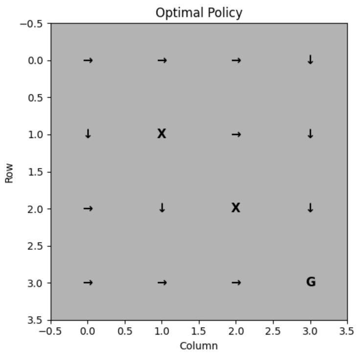
The solution for this problem is called a policy, which specifies what the agent should do for any state that the agent might reach. A policy is a mapping from states to actions that tells the agent what to do in each state:
Deterministic Policy:
Stochastic Policy:
where
Reinforcement Learning
The quality of the policy in a given state is measured by the expected utility of the possible environment histories generated by that policy. We can compute the utility of state sequences using additive (discounted) rewards as follows:
where
The expected utility of executing the policy
Reinforcement Learning
We can compare policies at a given state using their expected utilities:
The goal is to select the policy
The policy
Reinforcement Learning
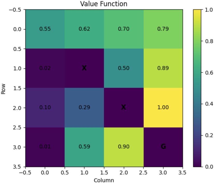
The utility function allows the agent to select actions by using the principle of maximum expected utility. The agent chooses the action that maximises the reward for the next step plus the expected discounted utility of the subsequent step:
The utility of a state is the expected reward for the next transition plus the discounted utility of the next state, assuming that the agent chooses the optimal action. The utility of a state
is given by:
This is called the Bellman Equation, after Richard Bellman (1957).
Reinforcement Learning
Reinforcement Learning
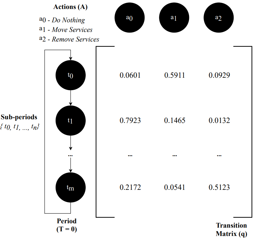
Another important quantity is the action-utility function or Q-function, which is the expected utility of taking a given action in a given state:
The Q-function tells us how good it is to take action
The optimal policy can be extracted from
Reinforcement Learning
Reinforcement Learning
Model-Based RL Agent
Model-Free RL Agent
- Knows transition model and reward function
- Can simulate outcomes before taking actions
- Value Iteration, Policy Iteration
- Unknown transition model and reward function
- Cannot simulate outcomes
- Q-Learning, DQN
Reinforcement Learning
Policy Iteration
Q-Value
DQN
Value-function
Model-based with guaranteed convergence for finite and discrete problems.
Q-function
Model-free and simple for small and discrete problems.

Neural Network
Model-free and complex for large and continuous problems.
Reinforcement Learning
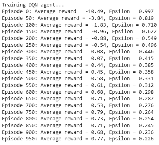
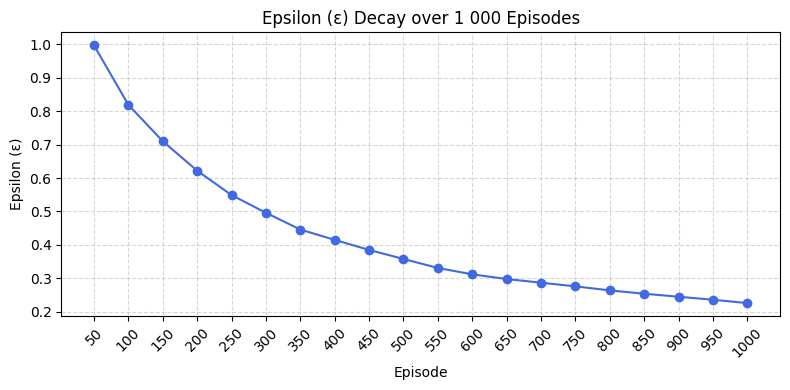
DQN Exercise Scenario

Reinforcement Learning

Reinforcement Learning
The Transformer Architecture
The Transformer Architecture
The Transformer is a deep neural network architecture based on the multi-head attention mechanism introduced by researchers at Google (Vaswani et al., 2017). The original goal was to improve machine learning translation tasks based on language modelling.
The Transformer Architecture

The Transformer Architecture
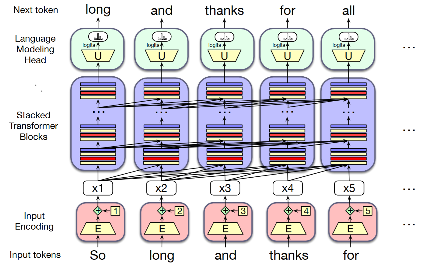
In Natural Language Processing (NLP), language modelling includes machine learning models (i.e., deep learning) to predict the next token in a sentence.
- Autoencoding tasks to fill in missing words (i.e., masked tokens)
- Autoregressive tasks to generate the next token in a sentence

The Transformer Architecture
The main idea is to pay attention to the context of each word in a sentence when modelling language. For example, if context is "Thanks for all the" and we want to know how likely the next word is "fish":

The Transformer Architecture
The main idea is to pay attention to the context of each word in a sentence when modelling language. For example, if context is "Thanks for all the" and we want to know how likely the next word is "fish":
We want to discover the probability distribution over a vocabulary
where

The Transformer Architecture
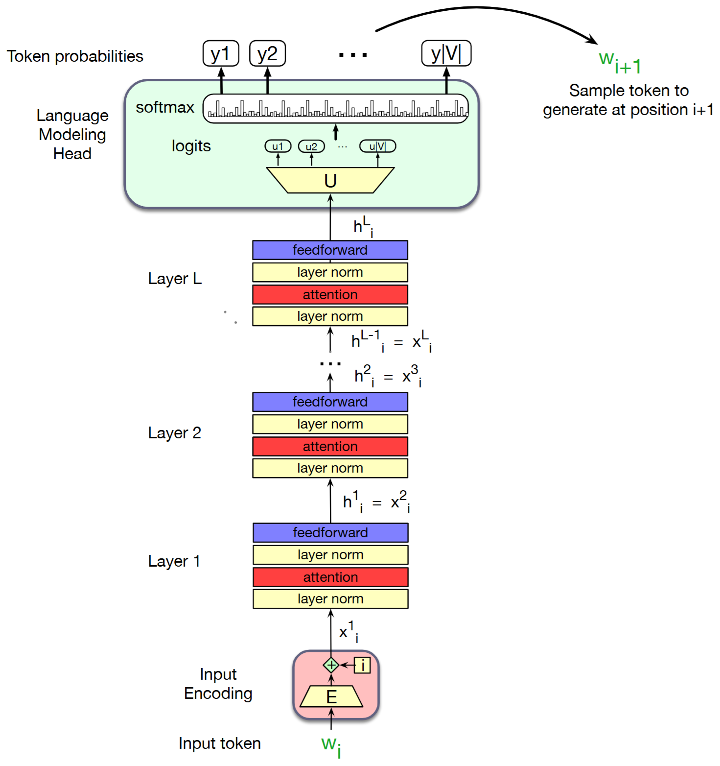
The transformer architecture solves this problem by:
- Tokenisation: Convert sentence into tokens.
- Input and Positional Embedding: Convert input tokens into ordered embedded vectors.
- Self-Attention: Determine the relevance of each word to others in the sequence.
- Feed-Forward Neural Network: Pass the attention outputs through a feed-forward neural network to consolidate learnt patterns.
- Residual Connections and Layer Normalisation: Apply residual connections and layer normalisation to stabilise and improve training.
- Output Layer: Use a linear layer followed by a softmax function to generate the final output probabilities.
The Transformer Architecture
1. Tokenisation: Convert sentence into tokens:

The Transformer Architecture
1. Tokenisation: Convert sentence into tokens:
For example, consider the sentence: "So long and thanks for".
Tokenisation of this sentence would result in the following tokens:
- "So"
- "long"
- "and"
- "thanks"
- "for"
Each word in the sentence is treated as an individual token.

The Transformer Architecture
2. Input and Positional Embedding: Convert input tokens into ordered embedded vectors:

The Transformer Architecture
2. Input and Positional Embedding: Convert input tokens into ordered embedded vectors:
Consider the tokens from the previous example: "So", "long", "and", "thanks", "for". Each token is converted into a vector using an embedding matrix. For instance:
- "So" -> [0.1, 0.3, 0.5, 0.7]
- "long" -> [0.2, 0.4, 0.6, 0.8]
- "and" -> [0.3, 0.5, 0.7, 0.9]
- "thanks" -> [0.4, 0.6, 0.8, 1.0]
- "for" -> [0.5, 0.7, 0.9, 1.1]
The embedding matrix has as many rows as words in a predefined vocabulary and as many columns as dimensions describing a word.

The Transformer Architecture
2. Input and Positional Embedding: Convert input tokens into ordered embedded vectors:
Positional encoding is then added to these vectors to incorporate the order of the tokens. For example:
- "So" -> [0.1, 0.3, 0.5, 0.7] + [0.0, 0.1, 0.2, 0.3]
- "long" -> [0.2, 0.4, 0.6, 0.8] + [0.1, 0.2, 0.3, 0.4]
- "and" -> [0.3, 0.5, 0.7, 0.9] + [0.2, 0.3, 0.4, 0.5]
- "thanks" -> [0.4, 0.6, 0.8, 1.0] + [0.3, 0.4, 0.5, 0.6]
- "for" -> [0.5, 0.7, 0.9, 1.1] + [0.4, 0.5, 0.6, 0.7]
Positional embeddings can be defined randomly. Each position having a random representation.
The resulting vectors are used as input to the transformer model, capturing both the meaning and position of each word. These are updated at training.

The Transformer Architecture
3. Self-Attention: Determine the relevance of each word to others in the sequence:

The Transformer Architecture
3. Self-Attention: Determine the relevance of each word to others in the sequence:
The meaning of a word represented by the embeddings is influenced by previous words. We need a mechanism (i.e., head) to transform the initial meaning of the words accordingly:

The Transformer Architecture
3. Self-Attention: Determine the relevance of each word to others in the sequence:
The meaning of a word represented by the embeddings is influenced by previous words. We need a mechanism (i.e., head) to transform the initial meaning of the words accordingly:
In the self-attention mechanism, each input embedding can play three distinct roles: query, key, and value.
- Query: As the current element compared to preceding inputs.
- Key: As a preceding input compared to the current element.
- Value: As a value of an element that gets weighted and summed up to compute the output of the current element.
We define three matrices to project each input into a representation of its role:
The Transformer Architecture
3. Self-Attention: Determine the relevance of each word to others in the sequence:
The meaning of a word represented by the embeddings is influenced by previous words. We need a mechanism (i.e., head) to transform the initial meaning of the words accordingly:

The Transformer Architecture
3. Self-Attention: Determine the relevance of each word to others in the sequence:
This is a multi-head attention mechanism where each head has its own set of key, query, and value matrices:
Each head focuses on different aspects of the language. One head can focus on the relationship between adjectives and nouns, another head can focus on the relation between verbs and subjects. These relationships transform the meaning of the input and are learnt from the data as model's parameters. The additional meaning is added to the original input as a residual connection.

The Transformer Architecture
4. Feed-Forward Neural Network: Pass the attention outputs through a feed-forward neural network to consolidate learnt patterns:

The Transformer Architecture
4. Feed-Forward Neural Network: Pass the attention outputs through a feed-forward neural network to consolidate learnt patterns:
Fully connected two-layer network
The input

The Transformer Architecture
5. Residual Connections and Layer Normalisation:

The Transformer Architecture
5. Residual Connections and Layer Normalisation:
Residual connections are used at different stages of the process to retain what the word originally meant whilst enriching it with context.

The Transformer Architecture
5. Residual Connections and Layer Normalisation:
Residual connections are used at different stages of the process to retain what the word originally meant whilst enriching it with context.
Layer normalisation is applied to keep the parameter values in a range that facilitate gradient descent.
In the equation above,

The Transformer Architecture
6. Output Layer: Use a linear layer followed by a softmax function to generate the final output probabilities:

The Transformer Architecture
6. Output Layer: Use a linear layer followed by a softmax function to generate the final output probabilities:
The linear layer applies a learnt weight matrix to the final hidden state, decoding the high-dimensional representation of the input sequence to a vector of logits, one for each possible output token.
The softmax function is applied to these logits to convert them into probabilities. The softmax function ensures that the output values are between 0 and 1 and that they sum up to 1, making them interpretable as probabilities. This step creates a probability distribution over the vocabulary.

The Transformer Architecture
The Transformer Architecture
Training Process:
The training process of a Transformer model involves:
- Loss Calculation: Compare the model's predictions to the actual outputs using a loss function, typically cross-entropy loss for classification tasks.
- Backpropagation: Compute the gradients of the loss with respect to the model parameters to adjust the model's weights.
The Transformer Architecture
Training Process:
The training process of a Transformer model involves:
- Optimization: An optimization algorithm, such as Adam, is used to update the model's weights based on the computed gradients.
- Iteration: Steps 4 to 7 are repeated for a number of epochs or until the model converges to a satisfactory performance level.
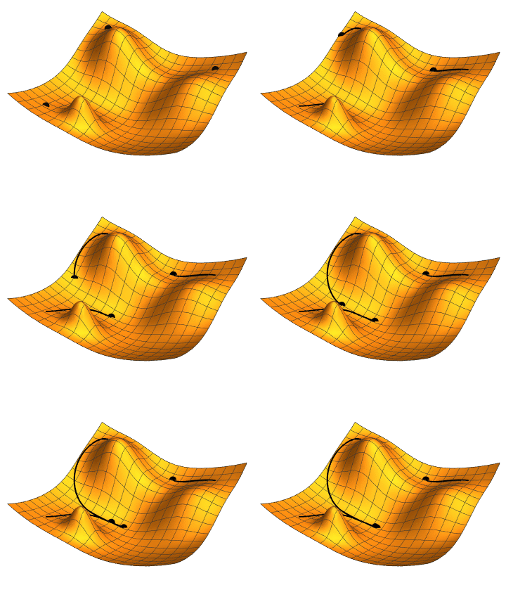
Throughout this process, various techniques such as dropout and learning rate scheduling may be employed to improve model performance and prevent overfitting.

The Transformer Architecture
Training Process:
The training process of a Transformer model can involve RL techniques for specific purposes:
- Reinforcement Learning from Human Feedback to align the model with human preferences.
- Task-Specific RL for fine-tuning for specific objectives like dialogue quality, summarisation, etc.
Large Language Models (LLMs)
Large Language Models (LLMs)
Large Language Models (LLMs)
Large Language Models (LLMs) are AI models designed to understand, generate, and manipulate human language. They are built using deep learning techniques and are usually based on the Transformer architecture and are trained on vast amounts of data to capture human language complexity. LLMs can perform a wide range of language tasks (e.g., text generation, classification, etc.).
AI History - Machine Learning Age (2001 - present)
Large Language Models (LLMs)

Large Language Models (LLMs)
- GPT-3: Known for generating human-like text, it can perform tasks such as translation, question answering, and text completion.
- BERT: Excels in understanding the context of words in a sentence, making it ideal for tasks like sentiment analysis and named entity recognition.
- T5 (Text-to-Text Transfer Transformer): Converts all NLP tasks into a text-to-text format, enabling it to handle tasks like summarisation and translation.
- RoBERTa: An optimised version of BERT, it improves performance on tasks like text classification and language inference.
- ...

Large Language Models (LLMs)
Large Language Models (LLMs)

Large Language Models (LLMs)
Fine-tuning continues the training of a pre-trained LLM (e.g., GPT-3, BERT, etc.) to perform tasks on a particular domain (e.g., healthcare).
Large Language Models (LLMs)

Large Language Models (LLMs)
It is similar to a neural network training:
- Data Collection: Gather a large and relevant dataset for the specific domain or task.
- Pre-processing: Clean and pre-process the data to ensure it is in a suitable format for training.
- Model Selection: Choose a pre-trained LLM that is most suitable for the task at hand.
- Supervised Learning: Prompt engineering, error calculation, and adjusting weights using gradient descent and backpropagation.
- Evaluation: Assess the performance of the fine-tuned model using appropriate metrics and validation datasets.
- Deployment: Deploy the fine-tuned model for use in real-world applications.

Large Language Models (LLMs)

Large Language Models (LLMs)
- Dataset Size: Typically requires tens of gigabytes to terabytes of data.
- RAM: Depends on the model size (i.e., number of parameters). At least 64GB or 128GB of RAM.
- GPU: High-performance GPUs such as NVIDIA A100 or V100 for faster training times.
- CPU: Multi-core processors, ideally with 16 cores or more, to handle data preprocessing and other tasks.
- Disk Space: Sufficient storage, often in the range of several terabytes, to accommodate datasets and model checkpoints.
- Network Bandwidth: High-speed internet connection for downloading datasets and model updates.

Large Language Models (LLMs)
Retrieval-Augmented Generation (RAG) is an alternative to fine-tuning that combines pre-trained LLMs with external knowledge sources. Instead of adapting the model to a specific domain, RAG retrieves relevant information from a database or knowledge base to enhance the model's responses in real-time.
Large Language Models (LLMs)
The process combines approaches from symbolic AI and databases:
- Data Collection: Gather a knowledge base that the RAG system can query.
- Pre-processing: Organise the knowledge base to ensure efficient retrieval and LLM integration.
- Model Selection: Choose a pre-trained LLM that can integrate with the retrieval system.
- Retrieval Integration: Using the knowledge base and the LLM in response to queries.
- Evaluation: Assess the performance of the RAG system by using appropriate metrics.
- Deployment: Deploy the RAG system for real-time applications, ensuring it can access and retrieve information efficiently.

Large Language Models (LLMs)

Large Language Models (LLMs)
- Knowledge Base Size: A comprehensive knowledge base can range from several gigabytes to terabytes.
- RAM: A minimum of 64GB is recommended to facilitate retrieval operations.
- GPU: Mid-range GPUs can suffice, but high-performance options like NVIDIA A100 can enhance performance.
- CPU: Multi-core processors for managing data preprocessing and retrieval tasks.
- Disk Space: Several terabytes may be necessary, depending on the data volume.
- Network Bandwidth: A high-speed internet connection for accessing external data sources and updating the knowledge base as needed.

Large Language Models (LLMs)
Prompt Engineering is a lightweight alternative to fine-tuning and RAG. Instead of changing model weights or building a retrieval pipeline, we craft instructions, examples, and constraints (the “prompt”) so that a frozen LLM performs the desired task.
Large Language Models (LLMs)
Typical prompt-engineering workflow:
- Task definition: Specify what output format and style you need.
- Baseline prompt: Write a clear instruction (zero-shot) or add 1-5 examples (few-shot).
- Iterate and test: Evaluate outputs, add system messages, or reorder examples to reduce errors and bias.
- Guardrails: Include refusals, safety clauses, or value alignment statements.
- Automation: Use prompt templates or tools like LangChain/LlamaIndex to inject dynamic context.
- Deployment: Store the prompt with version control and monitor performance over time.

Large Language Models (LLMs)
expected_format = """
Return your answer in JSON with the following keys:
{
  "title": string,          # concise headline (≤ 12 words)
  "summary": [string, ...]  # 3–5 bullet points
}
"""

article = """<ARTICLE TEXT HERE>"""

prompt = f"""
You are a helpful assistant.

TASK: Summarise the article below.

OUTPUT FORMAT (baseline)
{expected_format}

ARTICLE
""" + article

Large Language Models (LLMs)
import gemini

gemini.api_key = "YOUR_API_KEY"

response = gemini.Completion.create(
    engine="gemini-001",
    prompt=prompt,
    max_tokens=150,
    temperature=0.7
)
print(response.choices[0].text.strip())

Agentic AI
Agentic AI
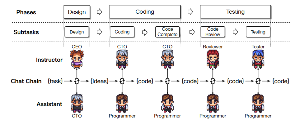
Agentic AI refers to systems that possess the capability to make autonomous decisions and take actions to achieve specific goals. This concept appeared with the emergence of LLMs and Generative AI.
Agentic AI

Agentic AI
Agentic AI
AI Agents have existed for decades, with active research communities and open challenges:
Agentic AI
AI Agents have existed for decades, with active research communities and open challenges:
- Reactive Agents: These agents perceive their environment and respond to changes.
- Deliberative Agents: These agents use symbolic reasoning and planning to make decisions.
- Hybrid Agents: Combining reactive and deliberative approaches.
- Multi-agent Systems: Systems where multiple agents interact or work together.
- Self-adaptive Systems: These systems can modify their behaviour in response to changes in their environment or internal state.
The difference is that LLM-based agents make the decision in Agentic AI frameworks.
Agentic AI
AI Agents have existed for decades, with active research communities and open challenges:
- Complex decision making processes
- Uncertainty management
- Agent coordination and scalability
- Algorithms robustness in dynamic environments
- Decision-making guarantees
- Control theory
- Social impact
- ...
The inclusion of LLM-based agents exacerbates some of these challenges.
Agentic AI
Large Language Models (LLMs)
Large Language Models (LLMs)
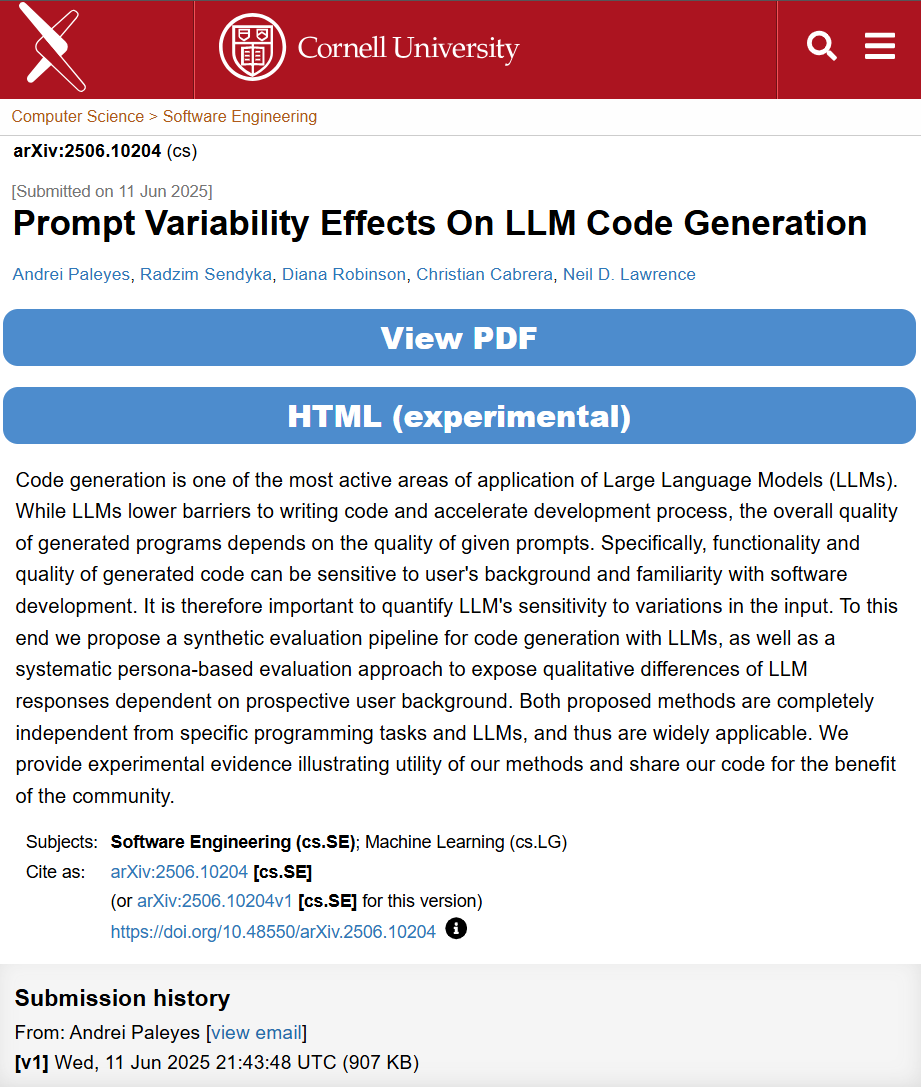
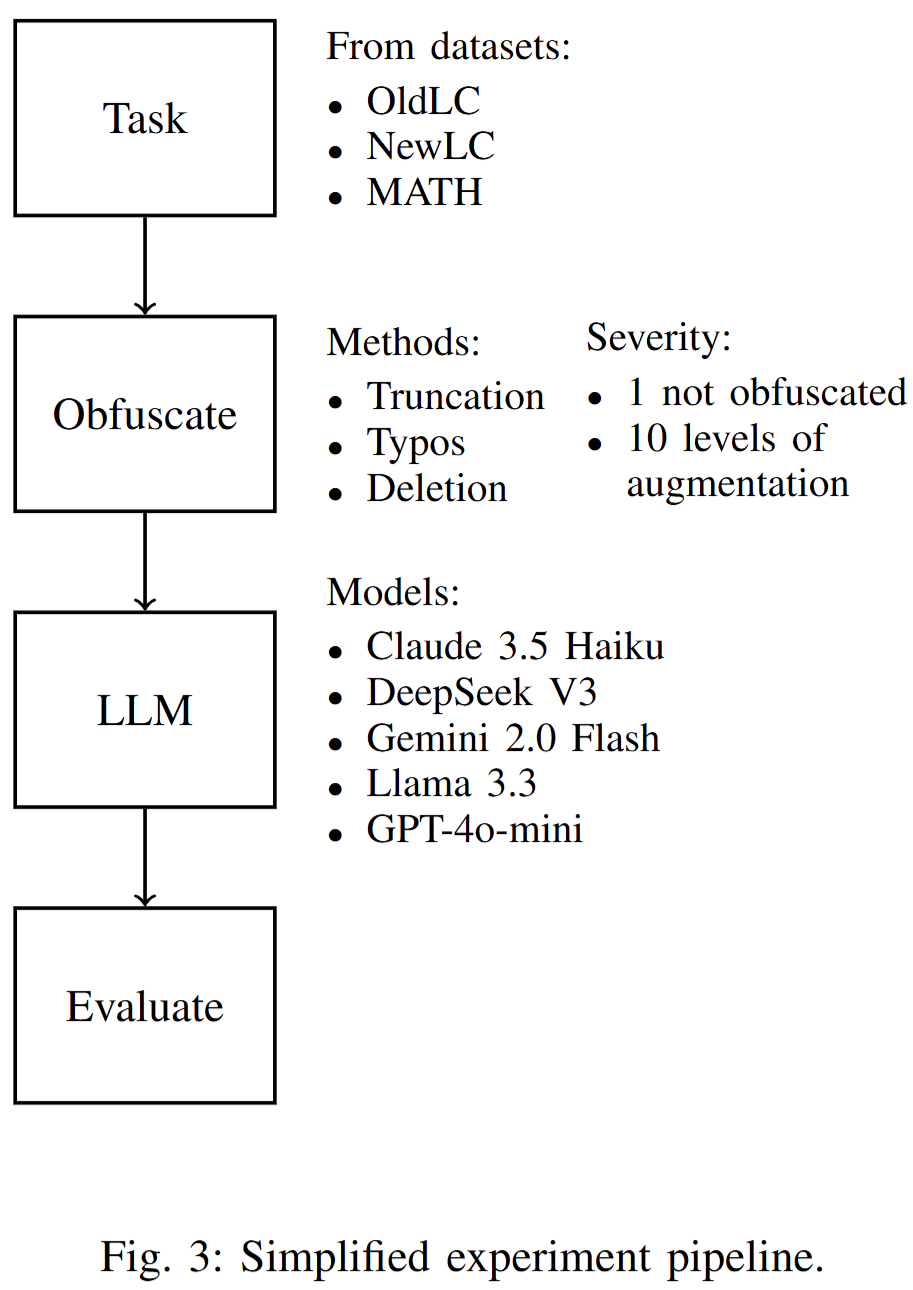
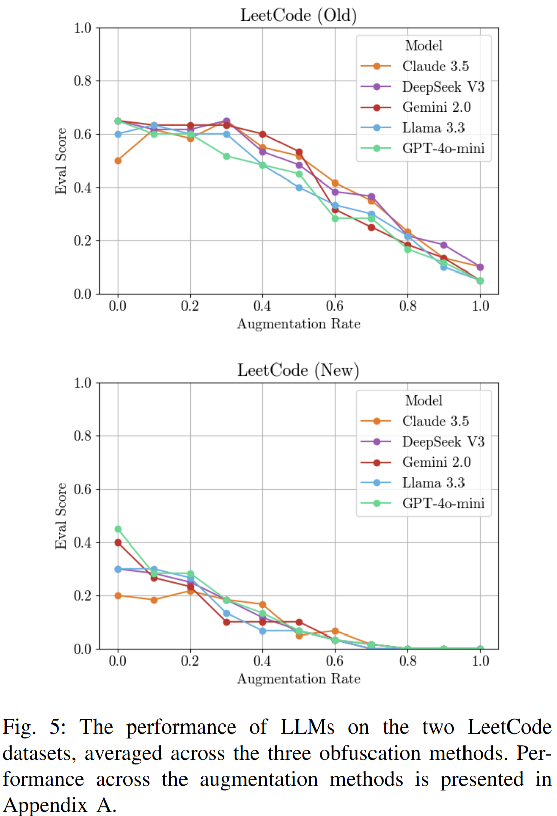
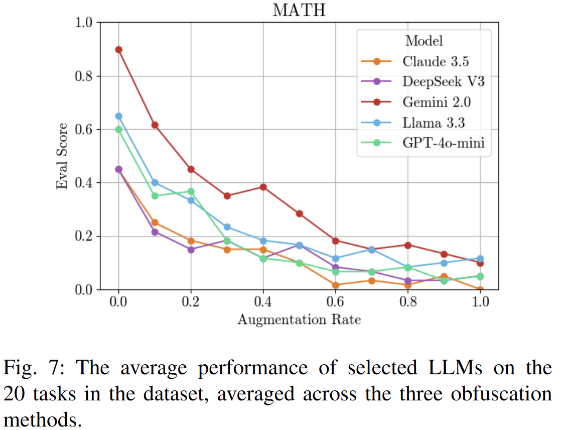
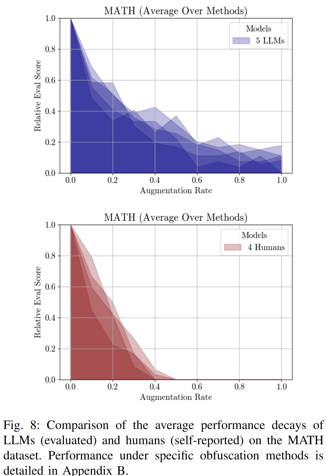
How sensitive are LLMs to changes in prompts when generating code?
Large Language Models (LLMs)
How sensitive are LLMs to changes in prompts when generating code?
'''
Write Python code to solve the following problem:

Given two arrays nums1 and nums2 of size m and n
respectively, return the medians of the two
arrays. The overall run time complexity should be
O(log (m+n)).
Constraints:
0 <= m <= 1000
0 <= n <= 1000
1 <= m + n <= 2000
-106 <= nums1[i], nums2[i] <= 106
'''
One change in the prompt was obfuscating the text by adding random noise:
'''
Write Python code to solve the following problem:

hJFFm two a8Gh4E se5Zuz GIJe! and mj<Cq of q&Xs m
and n %FE)2Xt(G#Oy, t$5 tDh the k$rJQH of the two
EPEˆ@W xGeX %E. The (gSFq<: run F(K@ DkN(;ss9r7 W
Bij>v be O (log (m + n) ).
K@jb$T = = n
0 <= m <= w000
0 <= n <= w000
1 <= m + n <= 1000
- 106 <= GHnZ@ [i ], jk,e@ [i] <= 106
'''
Large Language Models (LLMs)
Large Language Models (LLMs)
'''
Write Python code to solve the following problem:

hJFFm two a8Gh4E se5Zuz GIJe! and mj<Cq of q&Xs m
and n %FE)2Xt(G#Oy, t$5 tDh the k$rJQH of the two
EPEˆ@W xGeX %E. The (gSFq<: run F(K@ DkN(;ss9r7 W
Bij>v be O (log (m + n) ).
K@jb$T = = n
0 <= m <= w000
0 <= n <= w000
1 <= m + n <= 1000
- 106 <= GHnZ@ [i ], jk,e@ [i] <= 106
'''
Large Language Models (LLMs)
'''
Write Python code to solve the following problem:

hJFFm two a8Gh4E se5Zuz GIJe! and mj<Cq of q&Xs m
and n %FE)2Xt(G#Oy, t$5 tDh the k$rJQH of the two
EPEˆ@W xGeX %E. The (gSFq<: run F(K@ DkN(;ss9r7 W
Bij>v be O (log (m + n) ).
K@jb$T = = n
0 <= m <= w000
0 <= n <= w000
1 <= m + n <= 1000
- 106 <= GHnZ@ [i ], jk,e@ [i] <= 106
'''
Large Language Models (LLMs)
What can we conclude?
Large Language Models (LLMs)
What can we conclude?
- Are LLMs smarter than humans as they produce the correct answer even with obfuscated text?
Large Language Models (LLMs)
What can we conclude?
- Are LLMs smarter than humans as they produce the correct answer even with obfuscated text?
- Can LLM agents create their own language to fool us and dominate the world?
Large Language Models (LLMs)
What can we conclude?
- Are LLMs smarter than humans as they produce the correct answer even with obfuscated text?
- Can LLM agents create their own language to fool us and dominate the world?
- ...
Large Language Models (LLMs)
The actual conclusions are a bit more boring:
Large Language Models (LLMs)
The actual conclusions are a bit more boring:
- LLMs show signals of overfitting. They memorise the training data and generate text accordingly. They relate any pattern in the input with the training set and assign probabilities to next tokens.
Large Language Models (LLMs)
The actual conclusions are a bit more boring:
- LLMs show signals of overfitting. They memorise the training data and generate text accordingly. They relate any pattern in the input with the training set and assign probabilities to next tokens.
- LLM agents can communicate and exchange messages in formats humans cannot read. It threatens how we control autonomous systems as these are not transparent.
- We would expect a human to point out the issues in the text before even trying to provide an answer. Who is right?
Conclusions
Conclusions
Conclusions
Overview
- Transformer Architecture
- Self-Attention Mechanism
- Multi-Head Attention
- Large Language Models
- Fine-tuning, RAG, and Prompting
- Agentic AI
Conclusions
Overview
- Transformer Architecture
- Self-Attention Mechanism
- Multi-Head Attention
- Large Language Models
- Fine-tuning, RAG, and Prompting
- Agentic AI
Next Time
- ML Model Deployment
- MLOps
- AI as a Service
- AI-based Systems
