The Data Science Process

Machine Learning Pipeline

The Perceptron

Neural Networks
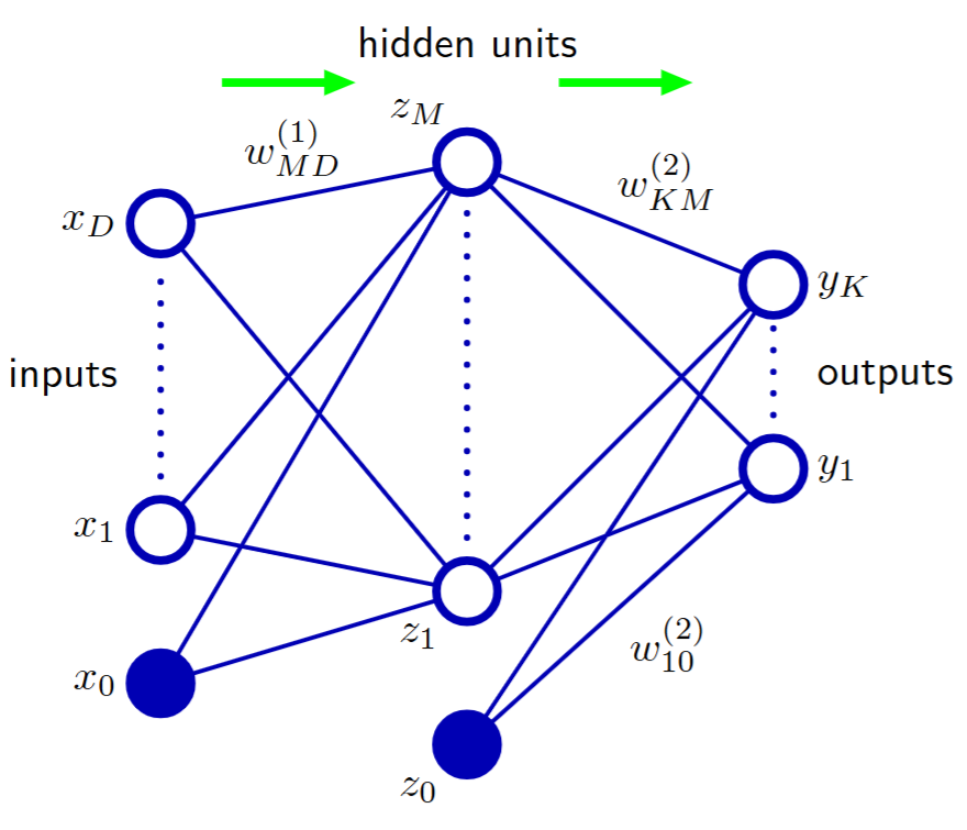
Neural networks extend the perceptron by introducing multiple layers of interconnected neurons (i.e., multi-layer perceptron), enabling the learning of complex, non-linear relationships in data.
Neural Networks
Neural Networks:
- Fix the number of basis functions in advance
- Basis functions are adaptive and their parameters can be updated during training
Training is costly but inference is cheap.
Neural Networks
Key Components:
- Input Layer: Receives the input features
- Hidden Layers: Process information through weighted connections
- Output Layer: Produces the final prediction
- Activation Functions: Introduce non-linearity
Neural Networks
Feedforward Neural Network:
The overall network function combines these stages. For sigmoidal output unit activation functions, takes the form:
The bias parameters can be absorbed:
Neural Networks
Sigmoid Function:
Range:
Derivative:
Hyperbolic Tangent:
Range:
Derivative:
ReLU (Rectified Linear Unit):
Range:
Derivative:
Neural Networks
Training Process:
Given a training set of N example input-output pairs
Each pair was generated by an unknown function
We want to find a hypothesis

Neural Networks
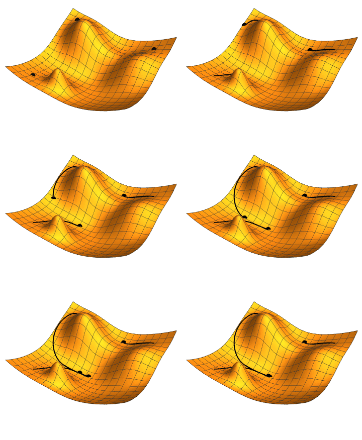
We choose any starting point and then compute an estimate of the gradient and move a small amount in the steepest downhill direction, repeating until we converge on a point in the weight space with (local) minima loss.
Gradient Descent Algorithm:
Initialise w
repeat
    for each w[i] in w
        Compute gradient: g = ∇Loss(w[i])
        Update weight:   w[i] = w[i] - α * g
until convergence
The size of the step is given by the parameter α, which regulates the behaviour of the gradient descent algorithm. This is a hyperparameter of the regression model we are training, usually called learning rate.
Neural Networks

Error Backpropagation Algorithm:
1. Forward Pass: Compute all activations and outputs for an input vector.
2. Error Evaluation: Evaluate the error for all the outputs using:
3. Backward Pass: Backpropagate errors for each hidden unit in the network using:
4. Derivatives Evaluation: Evaluate the derivatives for each parameter using:
Neural Networks

Gradient Descent Update Rule:
Where
Deep Learning
Hyperparameters Tuning
Hyperparameter Tuning
Hyperparameter Tuning
Hyperparameters tuning involves the process of optimising the parameters that govern the training process of a machine learning model, such as learning rate, number of layers, batch size, and number of epochs, to improve its performance and accuracy.
Hyperparameter Tuning
There is not a straight single answer to determine the "right" hyperparameter values.
Hyperparameter Tuning
There is not a straight single answer to determine the "right" hyperparameter values. But, experts follow similar steps:
- Become one with the data
- Set up the end-to-end training/evaluation skeleton
- Start with a simple model. For most of the tasks, a fully-connected neural network with one hidden layer.
- Implement a complex model that overfits and regularise
- Tune the hyperparameters
- Continue training
See more in Karpathy's recipe, and Tobin's lecture.
Hyperparameter Tuning
In the process, you should combine the methods previously discussed like preprocessing, feature engineering, normalising inputs, parameters initialisation, etc.
Hyperparameter Tuning
In the process, you should combine the methods previously discussed like preprocessing, feature engineering, normalising inputs, parameters initialisation, etc.

Reinforcement Learning
Reinforcement Learning
Reinforcement learning is a computational approach to learning from interaction with an environment to achieve a goal through trial and error. An agent learns to make decisions by receiving rewards or penalties (i.e., reinforcements) for its actions.
Reinforcement Learning

Reinforcement Learning

The agent aims to maximise the rewards from its actions. Rewards can be immediate or sparse.
Reinforcement Learning

The agent aims to maximise the rewards from its actions. Rewards can be immediate or sparse.
Providing a reward signal is easier than providing labelled examples (i.e., supervised learning).
Reinforcement Learning

The agent aims to maximise the rewards from its actions. Rewards can be immediate or sparse.
Providing a reward signal is easier than providing labelled examples (i.e., supervised learning).
Reinforcement Learning
Reinforcement Learning
The RL framework is composed of:
- Agent: The learner and decision maker
- Environment: The world in which the agent operates
- State: Current situation of the environment
- Action: What the agent can do
- Reward: Feedback from the environment
Reinforcement Learning
The RL framework is composed of:
- Agent: The learner and decision maker
- Environment: The world in which the agent operates
- State: Current situation of the environment
- Action: What the agent can do
- Reward: Feedback from the environment
The environment is stochastic, meaning that the outcomes of actions taken by the agent in each state are not deterministic.
Reinforcement Learning
Markov Decision Process (MDP):
A mathematical framework for modeling sequential decisions problems for fully observable, stochastic environments. The outcomes are partly random and partly under the control of a decision maker.
Reinforcement Learning
Markov Decision Process (MDP):
A mathematical framework for modeling sequential decisions problems for fully observable, stochastic environments. The outcomes are partly random and partly under the control of a decision maker.
Reinforcement Learning
A MDP is a 4-tuple:
Reinforcement Learning
A MDP is a 4-tuple:
Where:
Reinforcement Learning
The transition model describes the outcome of each action in each state. Since the outcome is stochastic, we write:
Reinforcement Learning
The transition model describes the outcome of each action in each state. Since the outcome is stochastic, we write:
Transitions are Markovian: The probability of reaching
Uncertainty once again brings MDPs closer to reality when compared against deterministic approaches.
Reinforcement Learning
From every transition the agent receives a reward:
Reinforcement Learning
From every transition the agent receives a reward:
The agent wants to maximise the sum of the received rewards (i.e., utility function):
The utility function
Reinforcement Learning
The solution for this problem is called a policy, which specifies what the agent should do for any state that the agent might reach. A policy is a mapping from states to actions that tells the agent what to do in each state:
Deterministic Policy:
Reinforcement Learning
The solution for this problem is called a policy, which specifies what the agent should do for any state that the agent might reach. A policy is a mapping from states to actions that tells the agent what to do in each state:
Deterministic Policy:
Stochastic Policy:
where
Reinforcement Learning
The quality of the policy in a given state is measured by the expected utility of the possible environment histories generated by that policy. We can compute the utility of state sequences using additive (discounted) rewards as follows:
where
Reinforcement Learning
The quality of the policy in a given state is measured by the expected utility of the possible environment histories generated by that policy. We can compute the utility of state sequences using additive (discounted) rewards as follows:
where
The expected utility of executing the policy
Reinforcement Learning
We can compare policies at a given state using their expected utilities:
Reinforcement Learning
We can compare policies at a given state using their expected utilities:
The goal is to select the policy
The policy
Reinforcement Learning
The utility function allows the agent to select actions by using the principle of maximum expected utility. The agent chooses the action that maximises the reward for the next step plus the expected discounted utility of the subsequent step:
Reinforcement Learning
The utility function allows the agent to select actions by using the principle of maximum expected utility. The agent chooses the action that maximises the reward for the next step plus the expected discounted utility of the subsequent step:
The utility of a state is the expected reward for the next transition plus the discounted utility of the next state, assuming that the agent chooses the optimal action. The utility of a state
is given by:
This is called the Bellman Equation, after Richard Bellman (1957).
Reinforcement Learning
Another important quantity is the action-utility function or Q-function, which is the expected utility of taking a given action in a given state:
Reinforcement Learning
Another important quantity is the action-utility function or Q-function, which is the expected utility of taking a given action in a given state:
Reinforcement Learning
Another important quantity is the action-utility function or Q-function, which is the expected utility of taking a given action in a given state:
Then we have:
Reinforcement Learning
Another important quantity is the action-utility function or Q-function, which is the expected utility of taking a given action in a given state:
The Q-function tells us how good it is to take action
Reinforcement Learning
Another important quantity is the action-utility function or Q-function, which is the expected utility of taking a given action in a given state:
The Q-function tells us how good it is to take action
The optimal policy can be extracted from
Reinforcement Learning
Reinforcement Learning
Model-Based RL Agent
Model-Free RL Agent
Reinforcement Learning
Model-Based RL Agent
Model-Free RL Agent
- Knows transition model and reward function
- Can simulate outcomes before taking actions
- Value Iteration, Policy Iteration
- Unknown transition model and reward function
- Cannot simulate outcomes
- Q-Learning, DQN
Reinforcement Learning
Policy Iteration is a model-based reinforcement learning algorithm that alternates between policy evaluation and policy improvement to find the optimal policy.
Reinforcement Learning
Policy Iteration is a model-based reinforcement learning algorithm that alternates between policy evaluation and policy improvement to find the optimal policy.
Finds the optimal policy through iterative refinement:
- Requires a model of the environment (transition and reward functions)
- Guaranteed to converge to the optimal policy
- Works with finite state and action spaces

Reinforcement Learning
Policy Iteration consists of two main phases that alternate until convergence:
Reinforcement Learning
Policy Iteration consists of two main phases that alternate until convergence:
1. Policy Evaluation: Compute the value function for the current policy:
Reinforcement Learning
Policy Iteration consists of two main phases that alternate until convergence:
1. Policy Evaluation: Compute the value function for the current policy:
2. Policy Improvement: Update the policy to be greedy with respect to the current value function:
Reinforcement Learning
Policy Iteration Algorithm:
The algorithm iteratively improves the policy by alternating between evaluation and improvement steps until convergence to the optimal policy.
Reinforcement Learning
Policy Iteration Algorithm:
The algorithm iteratively improves the policy by alternating between evaluation and improvement steps until convergence to the optimal policy.
The optimal policy maximizes the expected cumulative reward by selecting actions that lead to the highest Q-values.
Policy iteration guarantees convergence to the optimal policy through the principle of policy improvement.
Reinforcement Learning
Policy Iteration Algorithm:
Initialise policy π randomly
Repeat until convergence:
    // Policy Evaluation
    Repeat until convergence:
        For each state s:
            V(s) = Σ P(s'|s,π(s)) [R(s,π(s),s') + γV(s')]
    // Policy Improvement
    policy_stable = true
    For each state s:
        old_action = π(s)
        π(s) = argmaxₐ Σ P(s'|s,a) [R(s,a,s') + γV(s')]
        If old_action ≠ π(s):
            policy_stable = false
    If policy_stable:
        break
Convergence Properties:
- Monotonic Improvement: Each iteration improves the policy
- Finite Convergence: Guaranteed to converge in finite steps
- Optimal Policy: Converges to the optimal policy π*
- Bellman Optimality: Final policy satisfies Bellman optimality equations
Reinforcement Learning
Policy Iteration Limitations:

Reinforcement Learning
Policy Iteration Limitations:
- Model Dependency: Requires complete knowledge of the environment's transition and reward functions.
- Computational Cost: Policy evaluation can be expensive for large state spaces, requiring iterative computation.
- Discrete Spaces: Designed for finite state and action spaces, not suitable for continuous environments.
- Memory Requirements: Needs to store value functions and policies for all states.

Reinforcement Learning
Q-learning is a model-free reinforcement learning algorithm that learns the optimal action-value function directly from experience by interacting with the environment.
Finds the optimal policy by learning the Q-function:
- Does not require a model of the environment (transition or reward function)
- Can be used in stochastic and unknown environments

Reinforcement Learning
At each step, the agent updates its estimate of the Q-function for a state and action using the observed reward and the maximum estimated value of the next state. The update rule is defined as follows:
where:
Reinforcement Learning

Reinforcement Learning
Q-Learning Algorithm:
Initialize Q(s, a) arbitrarily for all s, a
Repeat (for each episode):
    Initialize state s
    Repeat (for each step of episode):
        a ← π(s)
        // Act according to a
        r ← = R(s, a, s')
        Q(s, a) ← update(Q, s, a, s', r)
        s ← s'
    until s is terminal

Reinforcement Learning
Q-Learning Algorithm:
Initialize Q(s, a) arbitrarily for all s, a
Repeat (for each episode):
    Initialize state s
    Repeat (for each step of episode):
        a ← π(s)
        // Act according to a
        r ← = R(s, a, s')
        Q(s, a) ← update(Q, s, a, s', r)
        s ← s'
    until s is terminal
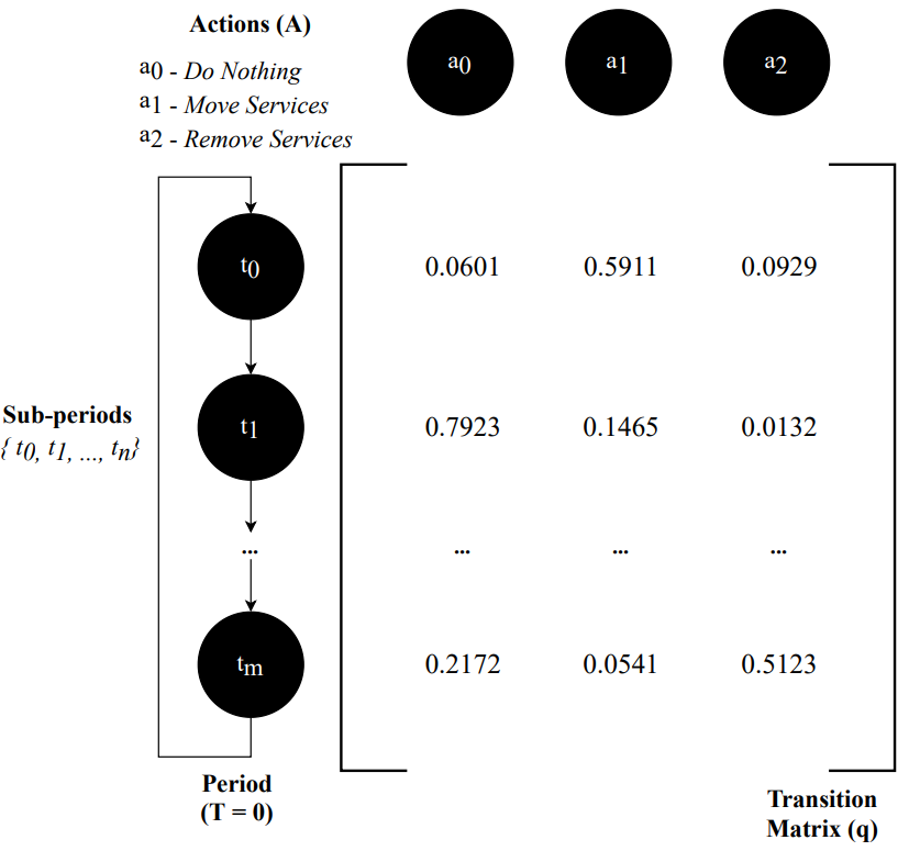
The agent must balance exploring new actions to discover their value and exploiting known actions to maximize reward.
ε-Greedy Policy:
Reinforcement Learning
Q-Learning Limitations:

Reinforcement Learning
Q-Learning Limitations:
- Scalability: Q-learning struggles with large state spaces as it requires a Q-value for every state-action pair, leading to high memory usage.
- Generalisation: Q-learning does not generalise well to unseen states since it relies on a discrete Q-table.
- Continuous State Spaces: Q-learning is not suitable for environments with continuous state spaces as it requires discretisation, which can lead to loss of information.
- Sample Inefficiency: Q-learning can be sample-inefficient, requiring many interactions with the environment to learn an optimal policy.

Reinforcement Learning
Deep Q-Networks (DQN) extend Q-learning to environments with large or continuous state spaces. It replaces the Q-table using neural networks to approximate the Q-function:
Reinforcement Learning
Deep Q-Networks (DQN) extend Q-learning to environments with large or continuous state spaces. It replaces the Q-table using neural networks to approximate the Q-function:
Reinforcement Learning
Deep Q-Networks (DQN) extend Q-learning to environments with large or continuous state spaces. It replaces the Q-table using neural networks to approximate the Q-function:
A main network approximates
Reinforcement Learning
Deep Q-Networks (DQN) extend Q-learning to environments with large or continuous state spaces. It replaces the Q-table using neural networks to approximate the Q-function:
A main network approximates
DQNs store past experiences
Reinforcement Learning
DQN Algorithm:
Initialise replay buffer D
Initialise Q-network with random weights w
Initialise target Q-network with weights w⁻ = w
Repeat (for each episode):
    Initialise state s
    Repeat (for each step of episode):
        a ← π(s)
        // Act according to a
        r ← = R(s, a, s')
        Store (s, a, r, s') in D
        For each (s, a, r, s') in mini_batch(D):
            y = r + γ maxₐ' Q(s', a'; w⁻)
        w ← gradient_descent((y - Q(s, a; w))²)
        Every C steps, update w⁻ ← w
        s ← s'
    until s is terminal
ε-Greedy Policy:
Reinforcement Learning
Policy Iteration
Q-Value
DQN
Reinforcement Learning
Policy Iteration
Q-Value
DQN
Value-function
Model-based with guaranteed convergence for finite and discrete problems.
Q-function
Model-free and simple for small and discrete problems.

Neural Network
Model-free and complex for large and continuous problems.
Reinforcement Learning
Reinforcement Learning

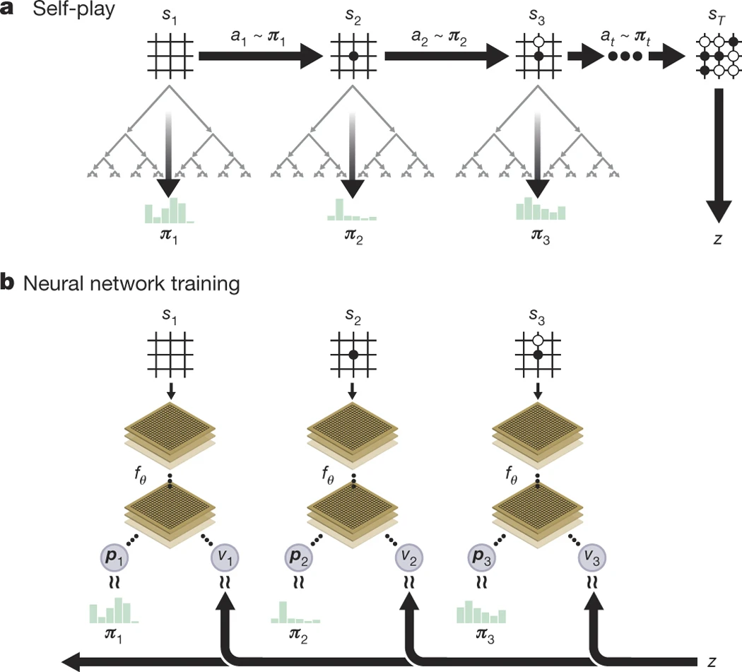
AlphaGo Zero combines key RL concepts:
- Self-play environment: Agent plays against itself (no human data needed)
- Policy network: Learns π(s) → probability distribution over actions
- Value network: Learns V(s) → probability of winning from state s
- Monte Carlo Tree Search: Uses policy/value to guide search
- Temporal difference learning: Updates based on game outcomes
- Experience replay: Stores and learns from self-play games
AI History - Machine Learning Age (2001 - present)
Conclusions
Conclusions
Overview
- Hyperparameters Tuning
- Reinforcement Learning
- Markov Decision Process
- Model-based RL
- Model-free RL
Conclusions
Overview
- Hyperparameters Tuning
- Reinforcement Learning
- Markov Decision Process
- Model-based RL
- Model-free RL
Next Time
- Attention Architecture
- Transformers
- Large Language Models (LLMs)
- LLMs APIs
- Prompt Engineering