The Data Science Process

Data Address
Data Address
After assessing the data (i.e., data assess), we need to use the data to address the problem in question. This process includes implementing a Machine Learning algorithm that creates a Machine Learning model.
Data Address

Data Address
A Machine Learning algorithm is a set of instructions that are used to train a machine learning model. It defines how the model learns from data and makes predictions or decisions. Linear regression, decision trees, and neural networks are examples of machine learning algorithms.

Data Address
A Machine Learning model is a program that is trained on a dataset and used to make predictions or decisions. The goal is to create a trained model that can generalise well to new, unseen data. For example, a trained model could predict house prices based on new input features.

Data Address
A Machine Learning algorithm uses the training process that goes from a specific set of observations to a general rule (i.e., induction). This process adjusts the Machine Learning model internal parameters to minimise prediction errors. For example, in a linear regression model, the algorithm adjusts the slope and intercept to minimise the difference between predicted and actual values.

Data Address
The parameters of Machine Learning models are adjusted according to the training data (i.e., seen data). For example, when training a model to predict house prices, the training data would include features like square footage, number of bedrooms, and location, along with their actual sale prices. The training data consists of vectors of attribute values.

Data Address
In classification problems, the prediction (i.e., model's output) is one of a finite set of values (e.g., sunny/cloudy/rainy or true/false). In the regression problems, the model's output is a number.

Data Address
Predictions can deviate from the expected values. Prediction errors are quantified by a loss function that indicates to the algorithm how far the prediction is from the target value. This difference is used to update the machine learning model's internal parameters to minimise the prediction errors. Common examples include Mean Squared Error for regression problems and Cross-Entropy for classification problems.

Data Address
Three types of feedback can be part of the inputs in our training process:
- Supervised Learning: The model is trained on labeled data to learn a mapping between inputs and the corresponding labels, so the model can make predictions on unseen data.
- Unsupervised Learning: The model is trained on unlabeled data, and it must find patterns in the data. The goal is to identify hidden structures or groupings in the data.
- Reinforcement Learning: The model learns by interacting with an environment and receiving rewards or penalties. The goal is to learn a policy that maximizes the reward.

Supervised Learning
The agent observes input-output pairs and learns a function that maps from input to output (label).
Supervised Learning
Given a training set of N example input-output pairs
Each pair was generated by an unknown function f.
The goal is to discover a function h that approximates the true function f.
Supervised Learning
Loss functions quantify the difference between predicted values and expected values (i.e., grounded truth).
Absolute value of the difference
Squared difference
Zero-One loss (classification error)
Supervised Learning
As P(x,y) is unknown, we can only estimate an empirical loss on a set of examples E of size N
Empirical loss for a hypothesis h using loss function L:
The best hypothesis h* is the one with the minimum empirical loss
Supervised Learning

Underfitting occurs when our hypothesis space H is too simple to capture the true function f
Even the best hypothesis h* in H will have high error because:
where epsilon is some small positive number.
Supervised Learning

Overfitting occurs when our hypothesis space H is too complex, leading to:
Low empirical loss but high generalisation loss:
The hypothesis h* memorizes the training examples instead of learning the true function f.
Supervised Learning

Regularisation transforms the loss function into a cost function that penalizes complexity to avoid overfitting.
Choosing the complexity function depends on the hypotheses space H. A good example for polynomials will be a function that returns the sum of the squares of coefficients.
Supervised Learning
Given the new cost function
The best hypothesis h* is the one that minimises the cost:
where λ is a hyperparameter that controls the trade-off between fitting the data and model complexity and serves as a conversion rate.
Alternatives to mitigate overfitting are feature selection, hyperparameter tuning, splitting dataset in training, validation, and test data (e.g., cross validation algorithm).
Regression
The regression problem involves predicting a continuous numerical value. Regression models approximate a function f that maps input features to a continuous output.
Regression Models

Linear Regression
Training Dataset
Hypothesis Space: All possible linear functions of continuous-valued inputs and outputs.
Hypothesis:
Loss Function:
Cost Function:
Regression Models


Regression Models
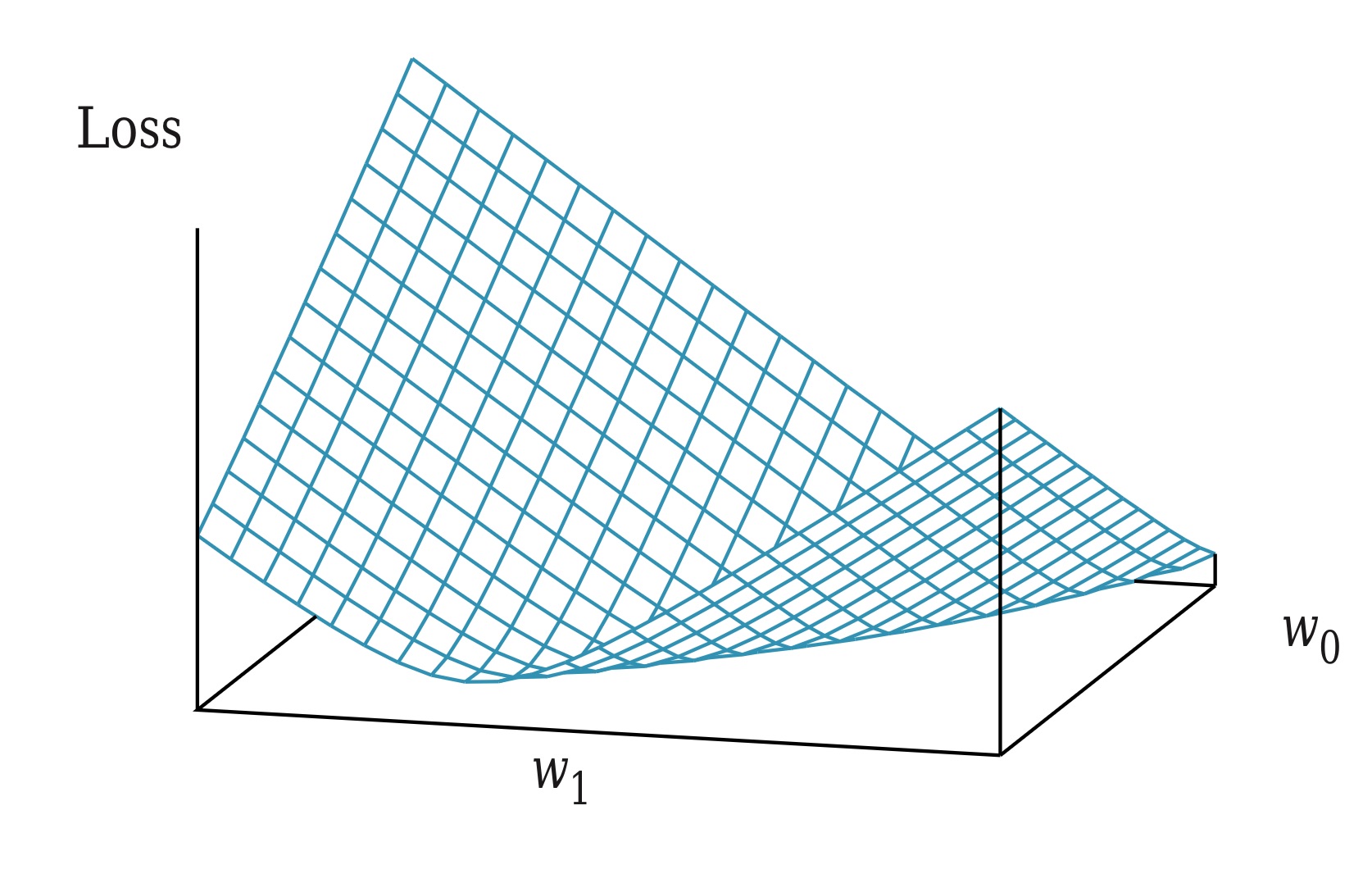
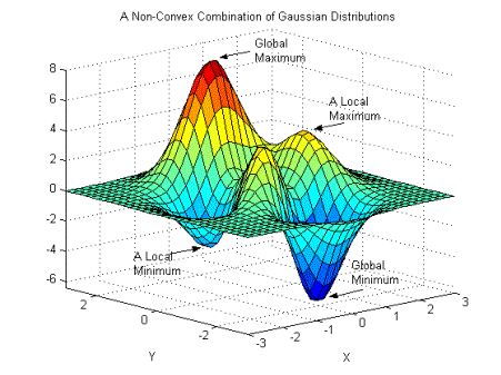
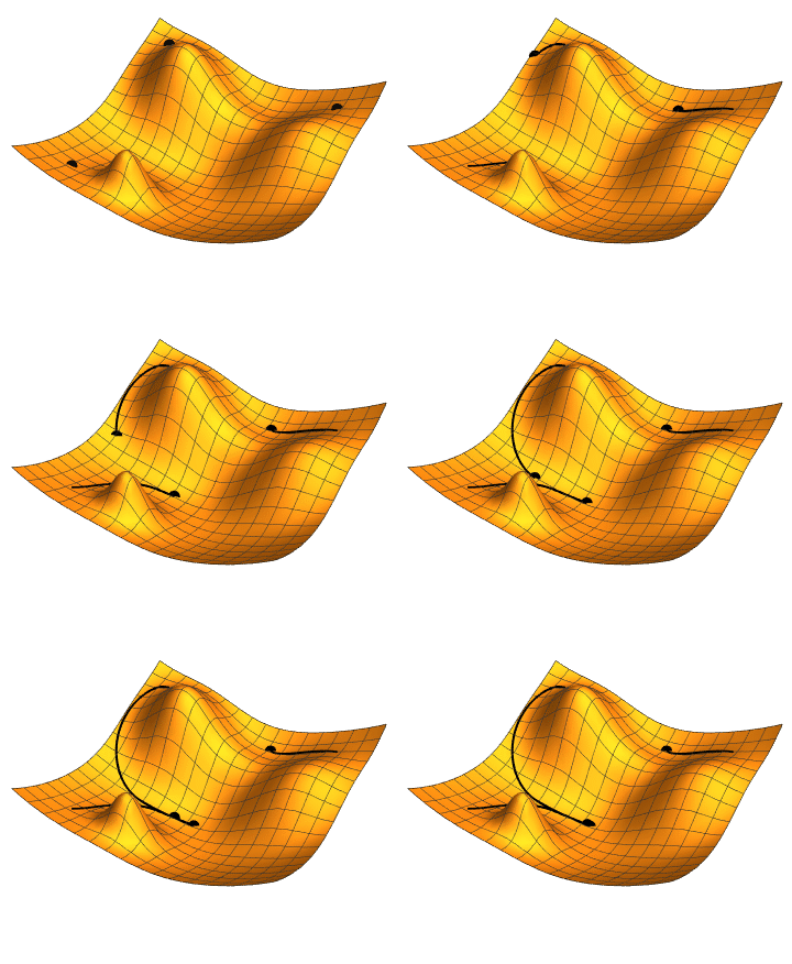
Regression Models

Linear Regression
Analytical Solution:
Gradient Descent Algorithm:
Initialize w randomly
repeat
    for each w[i] in w
        Compute gradient: g = ∇Loss(w[i])
        Update weight:   w[i] = w[i] - α * g
until convergence
Hyperparameters: Learning rate, number of epochs, and batch size.
Multivariate Linear Regression
Multivariate Linear Regression
Multivariate regression extends the simple linear model to handle multiple input features. The model learns a function that maps multiple input variables to a continuous output.
Multivariate Linear Regression
In these problems, each example is a n-element vector. The hypotheses space H now includes linear functions of multiple continuous-valued inputs and a single continuous output.
Multivariate Linear Regression
In these problems, each example is a n-element vector. The hypotheses space H now includes linear functions of multiple continuous-valued inputs and a single continuous output.
We want to find the
Multivariate Linear Regression
In these problems, each example is a n-element vector. The hypotheses space H now includes linear functions of multiple continuous-valued inputs and a single continuous output.
We want to find the
In vector notation:
Where
Multivariate Linear Regression
The loss function for multivariate regression is:
Multivariate Linear Regression
The loss function for multivariate regression is:
In matrix notation:
Where
Multivariate Linear Regression
Given the Loss function:
Multivariate Linear Regression
Given the Loss function:
We want to find
Multivariate Linear Regression
Given the Loss function:
We want to find
Taking the derivative with respect to
Multivariate Linear Regression
Given the Loss function:
We want to find
Taking the derivative with respect to
This leads to the normal equation:
Multivariate Linear Regression

Gradient Descent for Multivariate Regression
The gradient of the loss function is:
Multivariate Linear Regression

Gradient Descent for Multivariate Regression
The gradient of the loss function is:
Update rule for
Where
Probabilistic Interpretation of Linear Regression
Probabilistic Interpretation of Linear Regression
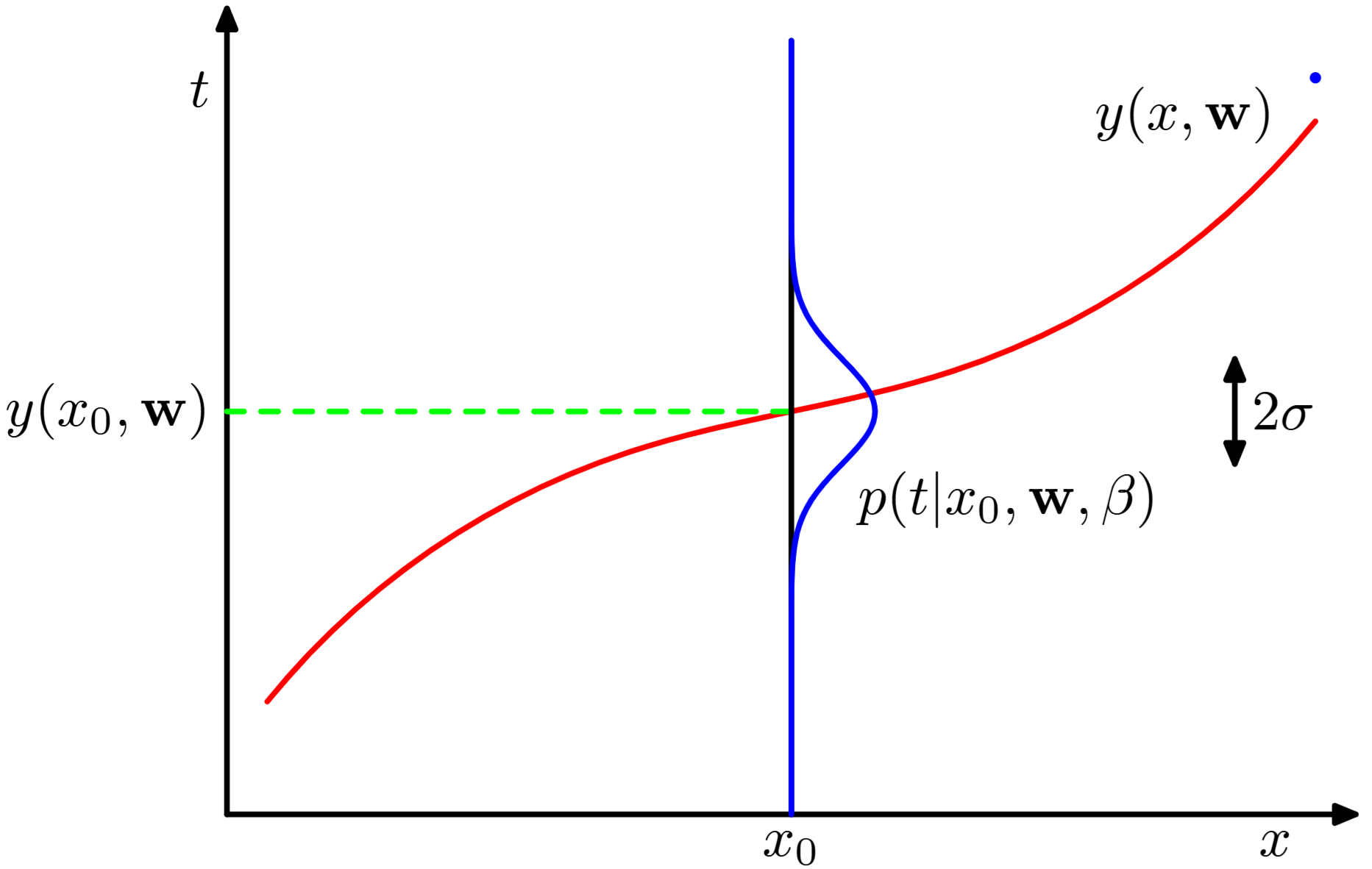
Linear regression can be interpreted from a probabilistic perspective, where we model the uncertainty in our predictions using probability distributions.
Probabilistic Interpretation of Linear Regression
Linear regression can be interpreted from a probabilistic perspective, where we model the uncertainty in our predictions using probability distributions.
Probabilistic Interpretation of Linear Regression
Instead of assuming deterministic relationships, we model the regression problem with the likelihood function:
Probabilistic Interpretation of Linear Regression
Instead of assuming deterministic relationships, we model the regression problem with the likelihood function:
The functional relationship between
Where
We want to find
Probabilistic Interpretation of Linear Regression
For linear regression, we have:
Where
Probabilistic Interpretation of Linear Regression
For linear regression, we have:
Where
So, given a training set of
Probabilistic Interpretation of Linear Regression
For linear regression, we have:
Where
So, given a training set of
The likelihood factorises according to:
Probabilistic Interpretation of Linear Regression
The likelihood function tells us how likely the observed data is given the specific parameters:
Probabilistic Interpretation of Linear Regression
The likelihood function tells us how likely the observed data is given the specific parameters:
We estimate
Probabilistic Interpretation of Linear Regression
Probabilistic Interpretation of Linear Regression
As before, a closed-form solution exists, which makes gradient descent unnecessary. We apply the log transformation to the likelihood function and minimise the negative log-likelihood.
Probabilistic Interpretation of Linear Regression
As before, a closed-form solution exists, which makes gradient descent unnecessary. We apply the log transformation to the likelihood function and minimise the negative log-likelihood.
We have that:
Probabilistic Interpretation of Linear Regression
Ignoring the constant terms:
Probabilistic Interpretation of Linear Regression
Ignoring the constant terms:
The loss function is defined as:
Where
Probabilistic Interpretation of Linear Regression
Minimising the Loss function is equivalent to minimising the sum of squared errors (MSE).
Probabilistic Interpretation of Linear Regression
Minimising the Loss function is equivalent to minimising the sum of squared errors (MSE).
As we did before, we compute the gradient of the Loss and equate it to zero:
Probabilistic Interpretation of Linear Regression
Minimising the Loss function is equivalent to minimising the sum of squared errors (MSE).
As we did before, we compute the gradient of the Loss and equate it to zero:
Solving the derivatives as we did before:
Probabilistic Interpretation of Linear Regression
The regression problem is considered as:
We want to maximise the likelihood function of the training data given the model parameters.
Closed-form solution for linear regression:
Where

Linear Basis Function Models
Linear Basis Function Models


Linear Basis Function Models
Linear basis function models extend linear regression by applying non-linear transformations to the input features while keeping the model linear in the parameters.
Linear Basis Function Models
The model becomes:
Where

Linear Basis Function Models
Polynomial basis:
Gaussian basis:
Sigmoid basis:

Linear Basis Function Models
If we apply a probabilistic interpretation, we need to maximise the likelihood of:
Linear Basis Function Models
If we apply a probabilistic interpretation, we need to maximise the likelihood of:
After a similar process (See Chapter 3 in Bishop, 2006), the loss function becomes:
Linear Basis Function Models
If we apply a probabilistic interpretation, we need to maximise the likelihood of:
After a similar process (See Chapter 3 in Bishop, 2006), the loss function becomes:
And the normal equation solution:
Linear Basis Function Models
Linear Basis Function Models
The design matrix
By using basis functions
Cross Validation
Cross-validation
Cross-validation is a technique for assessing model performance and preventing overfitting by evaluating the model on unseen data.
Cross-validation

Cross-validation
K-Fold Cross-validation divides the dataset into K equal parts:
for (int k = 1; k <= K; k++) {
    trainOnAllFoldsExcept(k);
    evaluateOnFold(k);
    recordPerformanceMetric(k);
}
calculateAveragePerformance(K);

Cross-validation
K-Fold Cross-validation divides the dataset into K equal parts:
for (int k = 1; k <= K; k++) {
    trainOnAllFoldsExcept(k);
    evaluateOnFold(k);
    recordPerformanceMetric(k);
}
calculateAveragePerformance(K);
Mathematically, for K-fold CV:
Where

Cross-validation
Leave-One-Out Cross-validation (LOOCV) is a special case where K = N:
Where

Linear Classifiers
Linear Classifiers
Linear classifiers are models that separate data into classes using a linear decision boundary. These classifiers are functions that can decide if an input (i.e., vectors of numbers) belong to a specific class or not.
Linear Classifiers

A decision boundary is a line (or a surface in higher dimensions) that separates data into classes.
Linear Classifiers

A decision boundary is a line (or a surface in higher dimensions) that separates data into classes.
The hypothesis is the result of passing a linear function through a threshold function:
Linear Classifiers

A decision boundary is a line (or a surface in higher dimensions) that separates data into classes.
The hypothesis is the result of passing a linear function through a threshold function:

Linear Classifiers
The optimal hypothesis is the one that minimises the loss function:
Where

Linear Classifiers
The optimal hypothesis is the one that minimises the loss function:
Where
Partial derivatives and gradient methods do not work. Instead, we apply perceptron learning rule.

Linear Classifiers
Perceptron update rule:
The rule is applied one example at a time, choosing examples at random (as in stochastic gradient descent).

Linear Classifiers
An alternative to the discrete threshold function is the logistic function, which is smooth and differentiable.

Linear Classifiers
An alternative to the discrete threshold function is the logistic function, which is smooth and differentiable.
Linear Classifiers
An alternative to the discrete threshold function is the logistic function, which is smooth and differentiable. The process of finding the optimal hypothesis is called logistic regression.
Where
Linear Classifiers
An alternative to the discrete threshold function is the logistic function, which is smooth and differentiable. The process of finding the optimal hypothesis is called logistic regression.
Where
Linear Classifiers
Following the gradient descent algorithm, the update rule is:
Linear Classifiers
Following the gradient descent algorithm, the update rule is:
The loss function is represented as a composition of functions:
Linear Classifiers
Following the gradient descent algorithm, the update rule is:
The loss function is represented as a composition of functions:
We need to differentiate the loss function using the chain rule to compute the gradients:
Linear Classifiers
Following the gradient descent algorithm, the update rule is:
Linear Classifiers
Following the gradient descent algorithm, the update rule is:
The resulting update rule after solving the partial derivatives:
The gradient descent algorithm is applied using this update rule.
Linear Classifiers

Gradient Descent for Logistic Regression
The gradient of the loss function is:
Update rule for
Where
The Perceptron
The Perceptron
The perceptron is one of the earliest and simplest artificial neural network models for binary classification.
The Perceptron
The Perceptron

The perceptron was simulated by Frank Rosenblatt in 1957 on an IBM 704 machine as a model for biological neural networks. The neural network was invented in 1943 by McCulloch & Pitts.
The Perceptron

The perceptron was simulated by Frank Rosenblatt in 1957 on an IBM 704 machine as a model for biological neural networks. The neural network was invented in 1943 by McCulloch & Pitts.
By 1962 Rosenblatt published the "Principles of Neurodynamics: Perceptrons and the Theory of Brain Mechanisms".
The Perceptron

The perceptron was simulated by Frank Rosenblatt in 1957 on an IBM 704 machine as a model for biological neural networks. The neural network was invented in 1943 by McCulloch & Pitts.
By 1962 Rosenblatt published the "Principles of Neurodynamics: Perceptrons and the Theory of Brain Mechanisms".
The Perceptron machine is named Mark I. It is a special-purpose hardware that implemented the perceptron supervised learning for image recognition.
The Perceptron

The Perceptron machine is named Mark I. It is a special-purpose hardware that implemented the perceptron supervised learning for image recognition.
The Perceptron

The Perceptron machine is named Mark I. It is a special-purpose hardware that implemented the perceptron supervised learning for image recognition.
- Input layer: An array of 400 photocells (20x20 grid) named "sensory units" or "input retina".
- Hidden Layer: 512 perceptrons named "association units" or "A-units".
- Output Layer: 8 perceptrons named "response units" or "R-units".
The Perceptron

The Perceptron

The Perceptron

The perceptron is a linear classifier model (i.e., linear discriminant), with hypothesis space defined by all the functions of the form:
The Perceptron

The perceptron is a linear classifier model (i.e., linear discriminant), with hypothesis space defined by all the functions of the form:
The function
The Perceptron

The perceptron is a linear classifier model (i.e., linear discriminant), with hypothesis space defined by all the functions of the form:
The function
We want to find
The Perceptron

The perceptron step function is not differentiable and the gradient is zero almost everywhere:
The Perceptron

The perceptron step function is not differentiable and the gradient is zero almost everywhere:
We need to derive the perceptron criterion. We know we are seeking parameters vector
And for features in
The Perceptron

The perceptron step function is not differentiable and the gradient is zero almost everywhere:
Using
The Perceptron

The perceptron step function is not differentiable and the gradient is zero almost everywhere:
Using
The loss function is:
The Perceptron

The loss function is:
The Perceptron

The loss function is:
The update rule for a missclassified input is:
The Perceptron
The perceptron learning algorithm is similar to the stochastic gradient descent.
Initialise weights w randomly
repeat
    for each training example (x, y)
        Compute prediction: y_pred = f(w·Φ(x))
        if y_pred ≠ y then
            Update weights: w = w + αΦ(x)y
until no misclassifications or max iterations
The Perceptron
import numpy as np

class Perceptron:
    def __init__(self, learning_rate=0.01, max_iterations=1000):
        self.learning_rate = learning_rate
        self.max_iterations = max_iterations
        self.weights = None
        self.bias = None
    def fit(self, X, y):
        n_samples, n_features = X.shape
        self.weights = np.zeros(n_features)
        self.bias = 0
        for _ in range(self.max_iterations):
            misclassified = 0
            for i in range(n_samples):
                prediction = self.predict(X[i])
                if prediction != y[i]:
                    self.weights += self.learning_rate * (y[i] - prediction) * X[i]
                    self.bias += self.learning_rate * (y[i] - prediction)
                    misclassified += 1
            if misclassified == 0:
                break
    def predict(self, x):
        return 1 if np.dot(self.weights, x) + self.bias >= 0 else 0
Python Implementation
The Perceptron
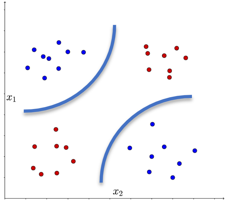
XOR Problem:
The perceptron cannot learn the XOR function because it's not linearly separable.
Other limitations:
- Only binary classification
- No probabilistic output
- The step function is not differentiable
- May oscillate for non-separable data
The Perceptron
The Perceptron

Conclusions
Overview
- Multivariate Linear Regression
- Probabilistic Interpretation of Linear Models
- Linear Basis Function Models
- Cross Validation
- Linear Classifiers
- The Perceptron
Conclusions
Overview
- Multivariate Linear Regression
- Probabilistic Interpretation of Linear Models
- Linear Basis Function Models
- Cross Validation
- Linear Classifiers
- The Perceptron
Next Time
- Neural Networks
- Deep Learning