The Data Science Process

Machine Learning Pipeline

Probabilistic Interpretation of Linear Regression
Linear regression can be interpreted from a probabilistic perspective, where we model the uncertainty in our predictions using probability distributions.
Probabilistic Interpretation of Linear Regression
Linear regression can be interpreted from a probabilistic perspective, where we model the uncertainty in our predictions using probability distributions.
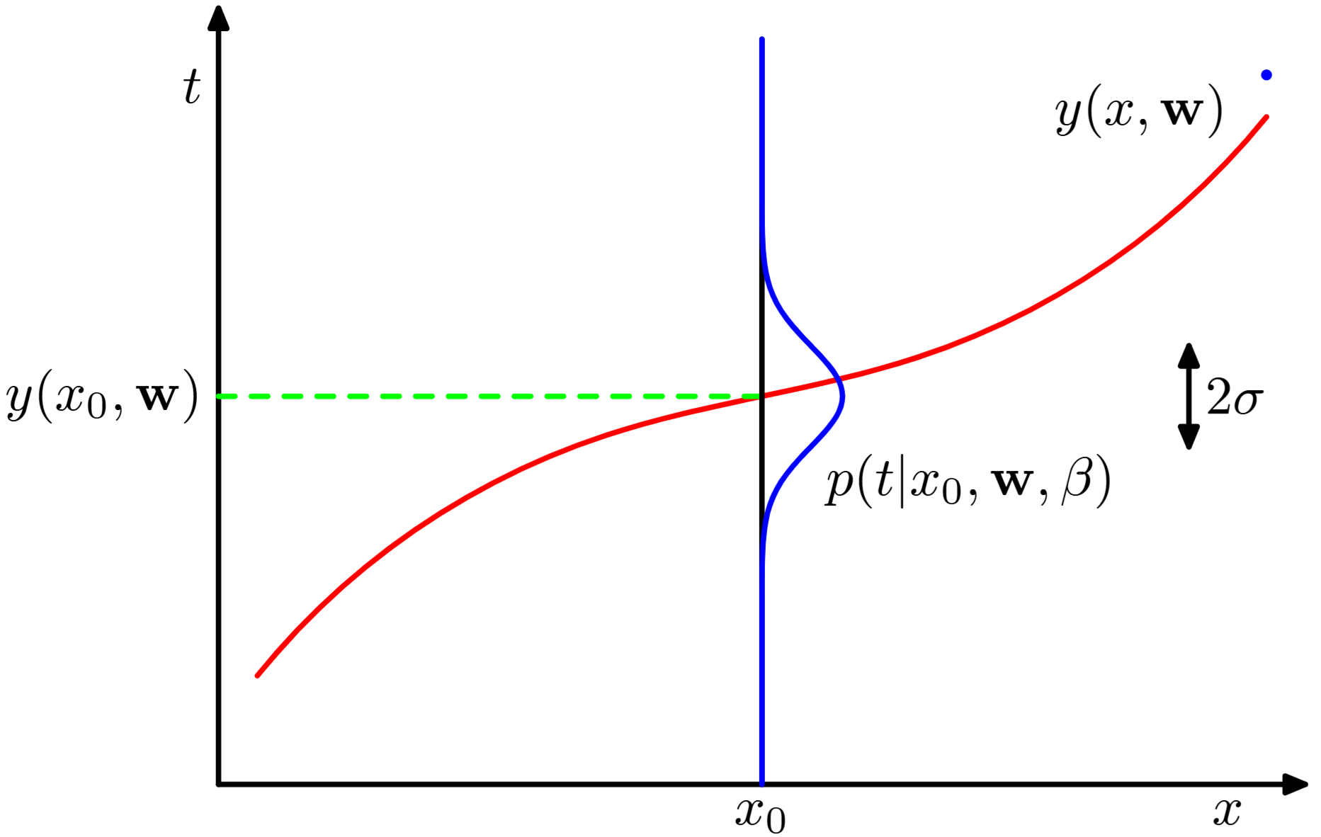
Probabilistic Interpretation of Linear Regression
Instead of assuming deterministic relationships, we model the regression problem with the likelihood function:
The functional relationship between
Where
We want to find
Probabilistic Interpretation of Linear Regression
For linear regression, we have:
Where
So, given a training set of
The likelihood factorises according to:
Probabilistic Interpretation of Linear Regression
The likelihood function tells us how likely the observed data is given the specific parameters:
We estimate
Linear Basis Function Models


Linear Basis Function Models
Linear basis function models extend linear regression by applying non-linear transformations to the input features while keeping the model linear in the parameters.
Linear Basis Function Models
The model becomes:
Where

Linear Basis Function Models
Polynomial basis:
Gaussian basis:
Sigmoid basis:

Linear Basis Function Models
If we apply a probabilistic interpretation, we need to maximise the likelihood of:
After a similar process (See Chapter 3 in Bishop, 2006), the loss function becomes:
And the normal equation solution:
Linear Basis Function Models
The design matrix
By using basis functions
The Perceptron
The perceptron is one of the earliest and simplest artificial neural network models for binary classification.
The Perceptron

The perceptron was simulated by Frank Rosenblatt in 1957 on an IBM 704 machine as a model for biological neural networks. The neural network was invented in 1943 by McCulloch & Pitts.
By 1962 Rosenblatt published the "Principles of Neurodynamics: Perceptrons and the Theory of Brain Mechanisms".
The Perceptron machine is named Mark I. It is a special-purpose hardware that implemented the perceptron supervised learning for image recognition.
The Perceptron

The Perceptron machine is named Mark I. It is a special-purpose hardware that implemented the perceptron supervised learning for image recognition.
- Input layer: An array of 400 photocells (20x20 grid) named "sensory units" or "input retina".
- Hidden Layer: 512 perceptrons named "association units" or "A-units".
- Output Layer: 8 perceptrons named "response units" or "R-units".
The Perceptron

The perceptron is a linear classifier model (i.e., linear discriminant), with hypothesis space defined by all the functions of the form:
The function
We want to find
The Perceptron

The perceptron step function is not differentiable and the gradient is zero almost everywhere:
We need to derive the perceptron criterion. We know we are seeking parameters vector
And for features in
The Perceptron

The perceptron step function is not differentiable and the gradient is zero almost everywhere:
Using
The loss function is:
The Perceptron

The loss function is:
The update rule for a missclassified input is:
The Perceptron
The perceptron learning algorithm is similar to the stochastic gradient descent.
Initialise weights w randomly
repeat
    for each training example (x, y)
        Compute prediction: y_pred = f(w·Φ(x))
        if y_pred ≠ y then
            Update weights: w = w + αΦ(x)y
until no misclassifications or max iterations
The Perceptron

Neural Networks
Neural Networks
Neural networks extend the perceptron by introducing multiple layers of interconnected neurons (i.e., multi-layer perceptron), enabling the learning of complex, non-linear relationships in data.
Neural Networks

Neural Networks

Previous models:
- Useful analytical and computational properties
- Limited application because of the curse of dimensionality
Neural Networks

Large scale problems require that we adapt the basis functions to the data.
Neural Networks
Large scale problems require that we adapt the basis functions to the data.
Neural Networks
Neural Networks:
- Fix the number of basis functions in advance
- Basis functions are adaptive and their parameters can be updated during training
Training is costly but inference is cheap.
Neural Networks
Key Components:
- Input Layer: Receives the input features
- Hidden Layers: Process information through weighted connections
- Output Layer: Produces the final prediction
- Activation Functions: Introduce non-linearity
Neural Networks
The Universal Approximation Theorem states that a neural network with one hidden layer can approximate any continuous function on a compact subset of ℝⁿ, given sufficient neurons in the hidden layer because neural networks form complex decision boundaries through the combination of linear transformations and non-linear activation functions.
Neural Networks
Feedforward Neural Network:
First, recall the general form of a linear model with nonlinear basis functions:
where

Neural Networks
Feedforward Neural Network:
First, recall the general form of a linear model with nonlinear basis functions:
where
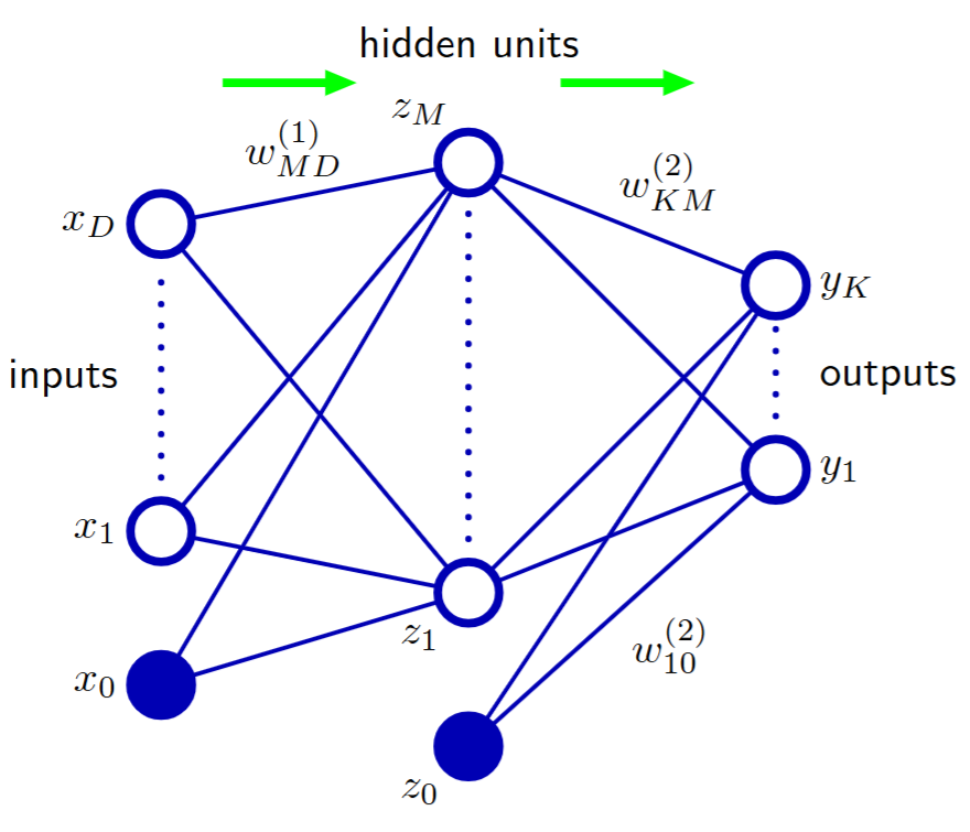
In neural networks, the basis functions themselves are parameterized and learned. The network is constructed as a sequence of transformations.
Neural Networks
Feedforward Neural Network:
1. Linear combination of inputs (first layer):
where

Neural Networks
Feedforward Neural Network:
1. Linear combination of inputs (first layer):
where
2. Nonlinear activation (hidden layer):
where

Neural Networks
Feedforward Neural Network:
1. Linear combination of inputs (first layer):
where
2. Nonlinear activation (hidden layer):
where

Neural Networks
Feedforward Neural Network:
3. Linear combination of hidden activations (output layer):
where

Neural Networks
Feedforward Neural Network:
3. Linear combination of hidden activations (output layer):
where
Optionally, the output activations

Neural Networks
Feedforward Neural Network:
The overall network function combines these stages. For sigmoidal output unit activation functions, takes the form:

Neural Networks
Feedforward Neural Network:
The overall network function combines these stages. For sigmoidal output unit activation functions, takes the form:
The bias parameters can be absorbed:

Neural Networks
Feedforward Neural Network:
The overall network function combines these stages. For sigmoidal output unit activation functions, takes the form:
The bias parameters can be absorbed:

Neural Networks
Activation functions introduce non-linearity into the network, enabling it to learn complex patterns and relationships.
Neural Networks
Neural Networks
Sigmoid Function:
Range:
Derivative:
Neural Networks
Sigmoid Function:
Range:
Derivative:
Hyperbolic Tangent:
Range:
Derivative:
Neural Networks
Sigmoid Function:
Range:
Derivative:
Hyperbolic Tangent:
Range:
Derivative:
ReLU (Rectified Linear Unit):
Range:
Derivative:
Neural Networks
Training Process:
Given a training set of N example input-output pairs

Neural Networks
Training Process:
Given a training set of N example input-output pairs
Each pair was generated by an unknown function

Neural Networks
Training Process:
Given a training set of N example input-output pairs
Each pair was generated by an unknown function
We want to find a hypothesis

Neural Networks
Training Process (regression problem):
Giving a probabilistic interpretation to the network outputs:
where

Neural Networks
Training Process (regression problem):
Giving a probabilistic interpretation to the network outputs:
where
For an i.i.d. training set, the likelihood function corresponds to:

Neural Networks
Training Process (regression problem):
For an i.i.d. training set, the likelihood function corresponds to:

Neural Networks
Training Process (regression problem):
For an i.i.d. training set, the likelihood function corresponds to:
As we saw in previous sessions, maximising the likelihood function is equivalent to minimising the sum-of-squares error function given by:

Neural Networks
Training Process (binary classification):
The network output is:
We use a single target variable

Neural Networks
Training Process (binary classification):
The network output is:
We use a single target variable

Neural Networks
Training Process (binary classification):
The network output is:
We use a single target variable
For an i.i.d. training, the error function is the cross-entropy error:

Neural Networks
Neural Networks

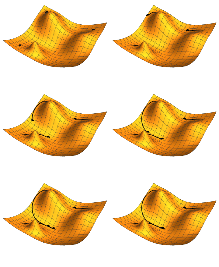
We choose any starting point and then compute an estimate of the gradient. We then move a small amount in the steepest downhill direction, repeating until we converge on a point in the weight space with (local) minima loss.
Gradient Descent Algorithm:
Initialize w
repeat
    for each w[i] in w
        Compute gradient: g = ∇Loss(w[i])
        Update weight:   w[i] = w[i] - α * g
until convergence
The size of the step is given by the parameter α, which regulates the behaviour of the gradient descent algorithm. This is a hyperparameter of the regression model we are training, usually called learning rate.
Neural Networks
Error backpropagation is an efficient algorithm for computing gradients in neural networks using the chain rule of calculus.
Neural Networks

Neural Networks

Error Backpropagation Algorithm:
Neural Networks

Error Backpropagation Algorithm:
1. Forward Pass: Compute all activations and outputs for an input vector.
Neural Networks

Error Backpropagation Algorithm:
1. Forward Pass: Compute all activations and outputs for an input vector.
2. Error Evaluation: Evaluate the error for all the outputs using:
Neural Networks

Error Backpropagation Algorithm:
1. Forward Pass: Compute all activations and outputs for an input vector.
2. Error Evaluation: Evaluate the error for all the outputs using:
3. Backward Pass: Backpropagate errors for each hidden unit in the network using:
Neural Networks

Error Backpropagation Algorithm:
1. Forward Pass: Compute all activations and outputs for an input vector.
2. Error Evaluation: Evaluate the error for all the outputs using:
3. Backward Pass: Backpropagate errors for each hidden unit in the network using:
4. Derivatives Evaluation: Evaluate the derivatives for each parameter using:
Neural Networks

Gradient Descent Update Rule:
Neural Networks

Gradient Descent Update Rule:
Neural Networks

Gradient Descent Update Rule:
Neural Networks

Gradient Descent Update Rule:
Where
Deep Learning
Deep Learning
Deep learning extends neural networks by using multiple hidden layers to learn hierarchical representations of data, enabling the automatic discovery of complex features.
Deep Learning
Deep Learning
Deep Learning
Key Characteristics:
- Multiple Hidden Layers: 3+ layers for deep architectures
- Hierarchical Features: Each layer learns increasingly abstract representations
- Automatic Feature Learning: No manual feature engineering required
- Representation Learning: Learns useful representations from raw data
Deep Learning
Vanishing and Exploding Gradients: In deep networks, gradients can become very small (vanishing) or very large (exploding) during backpropagation:
Deep Learning
Vanishing and Exploding Gradients: In deep networks, gradients can become very small (vanishing) or very large (exploding) during backpropagation:
- Proper Weight Initialization: Xavier/Glorot initialization
- Batch Normalization: Normalize activations during training
- Modern Optimizers: Adam, RMSprop with adaptive learning rates
- Regularisation: Dropout, L2, early stopping, and augmentation techniques
- Network Architectures: Different architectures for different problems
Deep Learning
Weight Initialization:
Xavier/Glorot Initialization:
He Initialization (for ReLU):
Where
Deep Learning
Input normalisation:
Where
Deep Learning
Modern Optimisers:
Optimisers train models by efficiently navigating the loss landscape to find optimal parameters. They help in accelerating convergence, avoiding local minima, and improving generalisation.
- Stochastic Gradient Descent (SGD): Updates parameters using a subset of data and reduces computation time.
- Adam: Adaptively adjust the learning rate for each parameter.
- ...

Deep Learning
Regularization Techniques:
Dropout: Randomly deactivate neurons during training
L2 Regularization: Add penalty to loss function
Early Stopping: Stop training when validation loss increases
Data Augmentation: Create additional training examples through transformations
Deep Learning
Network Architectures:
The architecture impacts the model's performance. The selection criteria includes: data type, task complexity, computational resources, generalisation needs
Deep Learning
Network Architectures:
The architecture impacts the model's performance. The selection criteria includes: data type, task complexity, computational resources, generalisation needs
- Residual Networks (ResNets): Allow gradients to flow through the network.

Deep Learning
Network Architectures:
The architecture impacts the model's performance. The selection criteria includes: data type, task complexity, computational resources, generalisation needs
- Residual Networks (ResNets): Allow gradients to flow through the network.
- Convolutional Neural Networks (CNNs): Used in image and video recognition tasks.
- Recurrent Neural Networks (RNNs): Applied in language modeling and sequence prediction tasks.
- Generative Adversarial Networks (GANs): Used for generating realistic data samples, such as images and audio.
Conclusions
Conclusions
Overview
- Neural Networks
- Forward Passing
- Backward Propagation
- Deep Learning
- Weights and Normalisation
- Optimisers and Regularisation
- ResNets, CNNs, and RNNs
Conclusions
Overview
- Neural Networks
- Forward Passing
- Backward Propagation
- Deep Learning
- Weights and Normalisation
- Optimisers and Regularisation
- ResNets, CNNs, and RNNs
Next Time
- Reinforcement Learning (RL)
- Markov Decision Processes (MDPs)
- Value Functions and Bellman Equations
- Policy and Value Iteration
- RL Algorithms
- Exploration vs. Exploitation
- Applications of RL