Supervised Learning
Given a training set of N example input-output pairs
Each pair was generated by an unknown function f
Supervised Learning
Given a training set of N example input-output pairs
Each pair was generated by an unknown function f
The goal is to discover a function h that approximates the true function f.
Supervised Learning
h is called a hypothesis. We need to search for h in a hypotheses space H of possible functions
Supervised Learning
h is called a hypothesis. We need to search for h in a hypotheses space H of possible functions
A consistent hypothesis maps each input to the corresponding grounded truth
Supervised Learning
h is called a hypothesis. We need to search for h in a hypotheses space H of possible functions
A consistent hypothesis maps each input to the corresponding grounded truth
We cannot expect exact match to the ground truth. We look for a best-fit function that generalises well.
The hypothesis h accurately predicts the outputs of unseen inputs (i.e., test set).
Supervised Learning
Our goal is to select a hypothesis h that will optimally fit future examples. Future examples will be like past examples (i.e., stationary assumption)
Supervised Learning
Our goal is to select a hypothesis h that will optimally fit future examples. Future examples will be like past examples (i.e., stationary assumption)
Each example has a the same prior probability distribution
Supervised Learning
Our goal is to select a hypothesis h that will optimally fit future examples. Future examples will be like past examples (i.e., stationary assumption)
Each example has a the same prior probability distribution
Each example is independent of previous examples
Examples that satisfy these equations are independent and identically distributed (i.e., iid).
Supervised Learning
Our goal is to select a hypothesis h that will optimally fit future examples. h is optimally fit if it minimises the error rate
Supervised Learning
Our goal is to select a hypothesis h that will optimally fit future examples. h is optimally fit if it minimises the error rate
The error rate is the proportion of times that h produces the wrong output for an example
Supervised Learning
Our goal is to select a hypothesis h that will optimally fit future examples. h is optimally fit if it minimises the error rate
The error rate is the proportion of times that h produces the wrong output for an example
Finding a good hypothesis implies choosing a good hypothesis space H and optimising or finding the best hypothesis h at training.
Supervised Learning
Loss functions quantify the difference between predicted values and expected values (i.e., grounded truth)
Supervised Learning
Loss functions quantify the difference between predicted values and expected values (i.e., grounded truth)
Absolute value of the difference
Supervised Learning
Loss functions quantify the difference between predicted values and expected values (i.e., grounded truth)
Absolute value of the difference
Squared difference
Supervised Learning
Loss functions quantify the difference between predicted values and expected values (i.e., grounded truth)
Absolute value of the difference
Squared difference
Zero-One loss (classification error)
Supervised Learning
We can generalise the loss by defining the prior probability distribution P(x,y) over examples
Supervised Learning
We can generalise the loss by defining the prior probability distribution P(x,y) over examples
Generalisation loss for a hypothesis h using loss function L:
Supervised Learning
We can generalise the loss by defining the prior probability distribution P(x,y) over examples
Generalisation loss for a hypothesis h using loss function L:
The best hypothesis h* is the one with the minimum expected generalisation loss
Supervised Learning
We can generalise the loss by defining the prior probability distribution P(x,y) over examples
Generalisation loss for a hypothesis h using loss function L:
The best hypothesis h* is the one with the minimum expected generalisation loss
But, P(x,y) is unknown in most cases.
Supervised Learning
As P(x,y) is unknown, we can only estimate an empirical loss on a set of examples E of size N
Supervised Learning
As P(x,y) is unknown, we can only estimate an empirical loss on a set of examples E of size N
Empirical loss for a hypothesis h using loss function L:
Supervised Learning
As P(x,y) is unknown, we can only estimate an empirical loss on a set of examples E of size N
Empirical loss for a hypothesis h using loss function L:
The best hypothesis h* is the one with the minimum empirical loss
Supervised Learning

Underfitting occurs when our hypothesis space H is too simple to capture the true function f
Supervised Learning

Underfitting occurs when our hypothesis space H is too simple to capture the true function f
Even the best hypothesis h* in H will have high error because:
where epsilon is some small positive number.
Supervised Learning

Overfitting occurs when our hypothesis space H is too complex, leading to:
Supervised Learning

Overfitting occurs when our hypothesis space H is too complex, leading to:
Low empirical loss but high generalisation loss:
The hypothesis h* memorizes the training examples instead of learning the true function f.
Supervised Learning

Regularisation transforms the loss function into a cost function that penalizes complexity to avoid overfitting
Supervised Learning

Regularisation transforms the loss function into a cost function that penalizes complexity to avoid overfitting
Choosing the complexity function depends on the hypotheses space H. A good example for polynomials will be a function that returns the sum of the squares of coefficients.
Supervised Learning
Given the new cost function
Supervised Learning
Given the new cost function
The best hypothesis h* is the one that minimises the cost:
where λ is a hyperparameter that controls the trade-off between fitting the data and model complexity and serves as a conversion rate.
Supervised Learning
Given the new cost function
The best hypothesis h* is the one that minimises the cost:
where λ is a hyperparameter that controls the trade-off between fitting the data and model complexity and serves as a conversion rate.
Alternatives to mitigate overfitting are feature selection, hyperparameter tuning, splitting dataset in training, validation, and test data (e.g., cross validation algorithm).
Regression
Regression
Regression
The regression problem involves predicting a continuous numerical value. Regression models approximate a function f that maps input features to a continuous output.
Regression
The hypotheses space H includes linear functions of continuous-valued inputs and outputs.
Regression Models
The hypotheses space H includes linear functions of continuous-valued inputs and outputs.
The simplest example is "fitting a straight line". The model learns the coefficients W
Regression Models
The hypotheses space H includes linear functions of continuous-valued inputs and outputs.
The simplest example is "fitting a straight line". The model learns the coefficients W

Regression Models


Regression Models
The simplest example is "fitting a straight line". The model learns the coefficients W
Finding the h that best fits the data is called linear regression.
Regression Models
The simplest example is "fitting a straight line". The model learns the coefficients W
Finding the h that best fits the data is called linear regression.
Finding the values of the weights w0 and w1 that minimise the empirical loss L2 (Squared Error).
Regression Models
Given the Loss(hw)
We want to find w*
Regression Models
Given the Loss(hw)
We want to find w*
We know that the loss is minimised when its partial derivatives with respect to w0 and w1 are zero.
Regression Models
We know that the loss is minimised when its partial derivatives with respect to w0 and w1 are zero.
Regression Models
We know that the loss is minimised when its partial derivatives with respect to w0 and w1 are zero.
Solving the partial derivatives
Regression Models
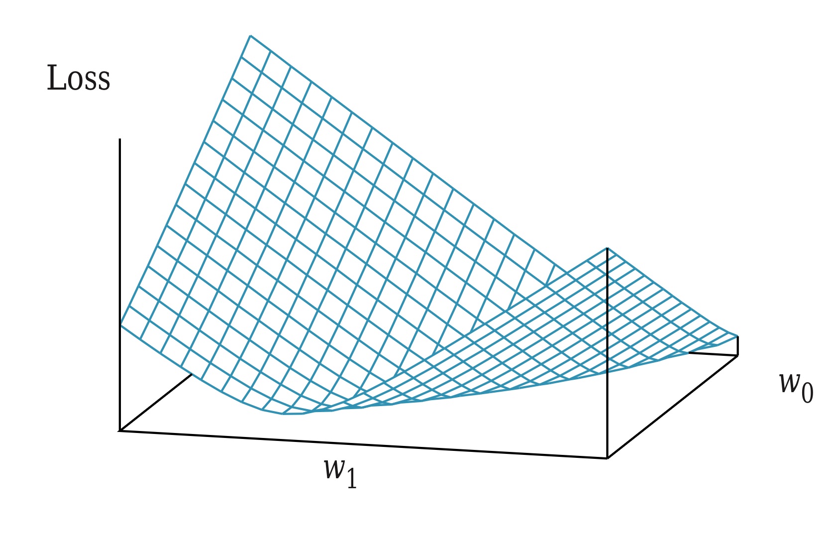
Regression Models

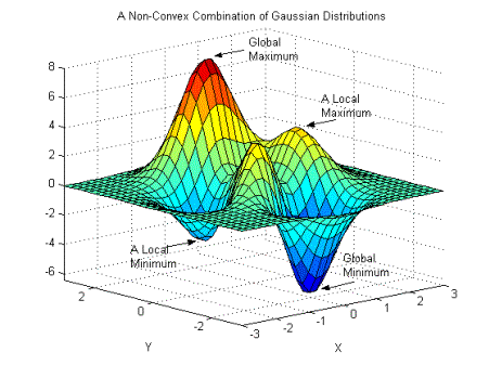
Regression Models


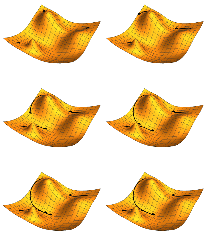
Regression Models

We choose any starting point and then compute an estimate of the gradient and move a small amount in the steepest downhill direction, repeating until we converge on a point in the weight space with (local) minima loss.
Gradient Descent Algorithm:
Initialize w randomly
repeat
    for each w[i] in w
        Compute gradient: g = ∇Loss(w[i])
        Update weight:   w[i] = w[i] - α * g
until convergence
The size of the step is given by the parameter α, which regulates the behaviour of the gradient descent algorithm. This is a hyperparameter of the regression model we are training, usually called learning rate.
Regression Models
Following with our "straight line" example, the update rule for w0 and w1 is
Regression Models
Following with our "straight line" example, the update rule for w0 and w1 is
The loss function is represented as a composition of functions.
Regression Models
Following with our "straight line" example, the update rule for w0 and w1 is
The loss function is represented as a composition of functions.
We need to differentiate the loss function step by step using the chain rule to compute the gradients.
Regression Models
Applying the chain rule to the loss function
Regression Models
Applying the chain rule to the loss function
Applying this to w0 and w1
Regression Models
The update rule for each weight in the "straight line" example is (folding 2 into α)
Regression Models
The update rule for each weight in the "straight line" example is (folding 2 into α)
For N training examples
These updates constitute the batch gradient descent. For the "straight line", this gradient descent is deterministic.
An epoch is defined as one complete pass through the entire dataset during the training process. Multiple epochs are needed for the model to converge to an optimal solution. Not enough epochs could generate underfitting. Too many epochs could generate overfitting. Another hyperparameter for the model.
Regression Models
Batch Gradient Descent
The algorithm updates W using the entire dataset in each iteration.
import numpy as np
def batch_gradient_descent(X, y, alpha=0.01, epochs=1000):
    """
    X: numpy array of shape (n_samples, n_features)
    y: numpy array of shape (n_samples,)
    alpha: learning rate
    epochs: number of passes over the data
    Returns: w (numpy array of shape (n_features,))
    """
    n_samples, n_features = X.shape
    w = np.zeros(n_features)
    for epoch in range(epochs):
        grad = [0] * len(w)
        for i in range(n_samples):
            x_i = X[i]
            y_i = y[i]
            prediction = dot(w, x_i)
            error = prediction - y_i
            for j in range(len(w)):
                grad[j] += error * x_i[j]
        for j in range(len(w)):
            grad[j] /= len(n_samples)
            w[j] -= alpha * grad[j]
    return w
Regression Models
Stochastic Gradient Descent
The algorithm updates W after computing the gradient for each training example.
import numpy as np
def stochastic_gradient_descent(X, y, alpha=0.01, epochs=1000):
    """
    X: numpy array of shape (n_samples, n_features)
    y: numpy array of shape (n_samples,)
    alpha: learning rate
    epochs: number of passes over the data
    Returns: w (numpy array of shape (n_features,))
    """
    n_samples, n_features = X.shape
    w = np.zeros(n_features)
    for epoch in range(epochs):
        for i in range(n_samples):
            x_i = X[i]
            y_i = y[i]
            prediction = np.dot(w, x_i)
            error = prediction - y_i
            for j in range(n_features):
                w[j] -= alpha * error * x_i[j]
    return w
Regression Models
Mini-batch Gradient Descent
The algorithm updates W after computing the gradient for a small batch of training examples (batch size m). The batch size is another hyperparameter.
import numpy as np
def mini_batch_gradient_descent(X, y, alpha=0.01, epochs=1000, batch_size=32):
    """
    X: numpy array of shape (n_samples, n_features)
    y: numpy array of shape (n_samples,)
    alpha: learning rate
    epochs: number of passes over the data
    batch_size: number of samples per batch
    Returns: w (numpy array of shape (n_features,))
    """
    n_samples, n_features = X.shape
    w = np.zeros(n_features)
    for epoch in range(epochs):
        indices = np.arange(n_samples)
        np.random.shuffle(indices)
        X_shuffled = X[indices]
        y_shuffled = y[indices]
        for start in range(0, n_samples, batch_size):
            end = start + batch_size
            X_batch = X_shuffled[start:end]
            y_batch = y_shuffled[start:end]
            y_pred = X_batch @ w
            error = y_pred - y_batch
            grad = X_batch.T @ error / len(X_batch)
            w -= alpha * grad
    return w
Regression Models

Linear Regression
Training Dataset
Hypothesis Space: All possible linear functions of continuous-valued inputs and outputs.
Hypothesis:
Loss Function:
Cost Function:
Regression Models

Linear Regression
Analytical Solution:
Gradient Descent Algorithm:
Initialize w randomly
repeat
    for each w[i] in w
        Compute gradient: g = ∇Loss(w[i])
        Update weight:   w[i] = w[i] - α * g
until convergence
Hyperparameters: Learning rate, number of epochs, and batch size.
Conclusions
Overview
- Statistical tests
- Supervised Learning
- Regression Problem
- Univariate Linear Regression
- Gradient Descent
Conclusions
Overview
- Statistical tests
- Supervised Learning
- Regression Problem
- Univariate Linear Regression
- Gradient Descent
Next Time
- Multivariate Linear Regression
- Linear Classification
- Non-parametric Models